80% of an AI project is data preparation. Yet, we spend 90% of our time talking about hyperparameters.
If you have ever trained a YOLO or Faster R-CNN model and watched the loss function plateau at a mediocre accuracy, your first instinct was probably to deepen the neural network or tweak the learning rate.
You were likely wrong.
The difference between a production-ready model and a failed POC often lies in how you draw a box. In this engineering guide, we are going to dissect the gritty reality of Data Annotation.
We will look at a real-world case study detecting electric wires and poles to show how shifting annotation strategies improved Model Average Precision (mAP) from a dismal 4.42% to a usable 72.61%, without changing the underlying algorithm.
The Challenge: The Thin Object Problem
Detecting cars or pedestrians is "easy" in modern CV terms. They are distinct, blocky shapes. But what happens when you need to detect Utility Wires?
- They are extremely thin (sometimes 1-2 pixels wide).
- They are diagonal (bounding boxes capture mostly background noise).
- They overlap with complex backgrounds (trees, buildings, sky).
Our team faced this exact problem. Here is how we engineered our way out of it using better data practices.
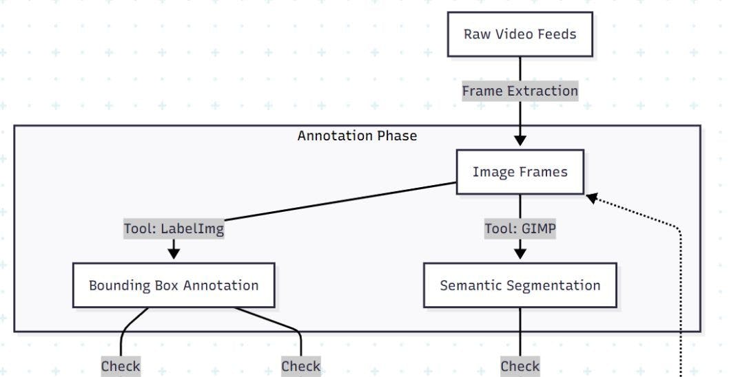
The Architecture: The Annotation Pipeline
Before we fix the data, let's establish the workflow. We moved from simple bounding boxes to semantic segmentation.
Phase 1: The Bounding Box Failure (Object Detection)
We started with LabelImg, the industry-standard open-source tool for Pascal VOC/YOLO annotations. We attempted to detect Wires and Poles.
Experiment A: The "Large Box" Approach
We drew a single bounding box around the entire span of a wire.
- Result: The model failed miserably.
- Why? A diagonal wire inside a rectangular box means 95% of the pixels inside that box are "Sky" or "Trees," not "Wire." The model learned to detect the background, not the object.
Experiment B: The "Small Box" Approach
We broke the wire down into multiple small, overlapping bounding boxes (like a chain).
- Result: Better, but still noisy.
- mAP: ~23.64%.
The "Clean Up" Pivot
We analyzed the False Negatives (missed detections) and found two major culprits in our dataset:
- Partial Visibility: Annotators had labeled poles that were <50% visible (hidden behind bushes). The model got confused about what a "pole" actually looked like.
- Loose Fitting: Annotators left small gaps between the object and the box edge.
The Fix:We purged the dataset. We removed any object with less than 50% visibility and tightened every bounding box to the exact pixel edge.
The Impact: mAP jumped to 72.61%.
Developer Takeaway: If your loss isn't converging, audit your "Partial Objects." If a human has to squint to see it, your model will hallucinate it.
Phase 2: The Segmentation Solution (Semantic Segmentation)
For objects like wires, bounding boxes are fundamentally flawed. We shifted to Semantic Segmentation, where every pixel is classified.
Surprisingly, we didn't use an expensive AI suite for this. We used GIMP (GNU Image Manipulation Program).
The Layering Strategy
To feed a segmentation model (like U-Net or Mask R-CNN), you need precise masks. Here is the GIMP workflow that worked:
- Layer 1 (Red): Wires. We used the "Path Tool" to stroke lines slightly thinner than the actual wire to ensure no background bleeding.
- Layer 2 (Green): Poles.
- Layer 3: Background.
**The Code: Converting Masks to Tensors \ Once you have these color-coded images, you need to convert them for training. Here is a Python snippet to convert a GIMP mask into a binary mask for training:
import cv2
import numpy as np

def process_mask(image_path):
    # Load the annotated image
    img = cv2.imread(image_path)

    # Define color ranges (e.g., Red for Wires)
    # OpenCV uses BGR format
    lower_red = np.array([0, 0, 200])
    upper_red = np.array([50, 50, 255])

    # Create binary mask
    wire_mask = cv2.inRange(img, lower_red, upper_red)

    # Normalize to 0 and 1 for the model
    wire_mask = wire_mask / 255.0

    return wire_mask

# Usage
mask = process_mask("annotation_layer.png")
print(f"Wire pixels detected: {np.sum(mask)}")
Best Practices: The "Do Not Do" List
Based on thousands of annotated images, here are the three cardinal sins of annotation that will ruin your model.
1. The Loose Box Syndrome
- The Mistake: Leaving "air" between the object and the box.
- The Consequence: The model learns that a "Pole" includes the slice of sidewalk next to it. When tested on a pole in the grass, it fails.
- The Fix: Boxes must be pixel-perfect tight.
2. The Edge Case Trap
- The Mistake: Drawing a box that touches the absolute edge of the image frame (0,0 coordinates).
- The Consequence: Many augmentation libraries (like Albumentations) glitch when boxes touch the border during rotation/cropping.
- The Fix: Always leave a 1-pixel buffer from the image edge if possible.
3. The Ghost Label
- The Mistake: Labeling an object that is occluded (e.g., a pole behind a billboard) because you know it's there.
- The Consequence: The model learns to hallucinate objects where none exist visually.
- The Fix: If it isn't visible, it isn't there. Do not annotate implied objects.
Tooling Recommendation
Which tool should you use?
|
Tool |
Best For |
Pros |
Cons |
|---|---|---|---|
|
LabelImg |
Object Detection |
Free, Fast, XML/YOLO export |
Bounding boxes only (No polygons) |
|
CVAT |
Segmentation |
Web-based, supports teams |
Steeper learning curve |
|
GIMP |
Pixel-Perfect Masks |
Extreme precision |
Manual, slow for large datasets |
|
VGG VIA |
Quick Polygons |
Lightweight, Runs offline |
UI is dated |
Conclusion
We achieved a 90%+ milestone in wire detection not by inventing a new transformer architecture, but by manually cleaning 50-100 pixel-range bounding boxes.
AI is not magic; it is pattern matching. If you feed it messy patterns, you get messy predictions. Before you fire up that H100 GPU cluster, open up your dataset and check your boxes.


