
Table Of Links
VI. RESULTS OF DECOMPOSITION’S APPLICATION
VII. CONCLUSION, ACKNOWLEDGMENTS AND REFERENCES
IV. METHODOLOGY
As mentioned previously, we have not identified a direct method to decompose a MAPF instance into multiple subproblems. Thus, we initiate the process with an initial decomposition, progressively refining it to generate smaller subproblems while ensuring that each step maintains solvability. We define two types of subproblems encountered in various stages: clusters, which have no restrictions on the order of solving, and levels, which impose limitations on the order of solving.
The decomposition of a MAPF instance involves three steps:
1, identifying all agent dependencies and establishing initial clusters based on them;
2, refining agent dependencies to bipartition clusters until they cannot be further divided into smaller clusters;
3, further refining agent dependencies to decompose clusters into levels and sorting; Step 1 and 2 are described in Section IV-A, and step 3 is described in Section IV-C. An overview of the decomposition process of a MAPF instance is depicted in Figure 1.
Following decomposition, we explore methods to solve subproblems independently and then combine their results to obtain a conflict-free solution for the original MAPF instance, as detailed in Section IV-D.
A. Decomposetion to clusters
The first step is to determine the connectivity graph Gc from a grid space CN and the related agents A. We then determine initial clusters based on the dependence paths derived from the connectivity graph.
Definition 4: Relevance of two agents: If an agent ai’s dependence path contains another agent aj ’s start or target, we consider those two agents as relevant, regardless of whether aj ’s dependence path contains ai’s start or target. It is noteworthy that the relevance of two agents is determined by their dependence paths, so whether two agents are relevant changes as their dependence paths change. For the three dependence paths mentioned before, agent 0 and agent 1 are relevant, while agent 2 is irrelevant to either of them.
Definition 5: Graph of agents’ relevance Ga: an undirected graph where nodes represent agents and edges represent whether two agents are relevant.
Definition 6: Cluster: a maximal connected subgraph (i.e., connected component) of Ga. Intuitively, a cluster is a set of agents from the raw MAPF instance, where any agents within it are only relevant to agents within the same set (based on their dependence paths). A cluster is denoted as r, and a set of clusters is denoted as R. Additionally, we refer to an agent set that constitutes a cluster as an independent agent set.
For the three dependence paths mentioned before, agent 0 and agent 1 form one cluster, while agent 2 forms another cluster.
An intuitive way to obtain clusters is by extracting clusters from the dependence paths that visit the fewest number of agents for each agent. We refer to such clusters as initial clusters.
However, it is evident that selecting dependence paths containing the fewest agents may not always result in the smallest possible clusters, as it does not consider how to guide dependence paths to avoid agents from other clusters.
There is room for decomposing these initial clusters into smaller ones by updating the dependence paths of agents (in implementation, we verify the existence of such paths rather than explicitly maintaining all agents’ dependence paths).
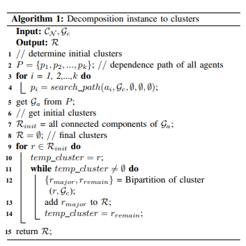
Thus, we propose a method to iteratively bipartition initial clusters until further subdivision is not possible, aiming to minimize the size of subproblems. More details about bipartitioning can be found in the following section. This process ensures the solvability of decomposition, and the more bipartitioning steps, the better the results obtained, although it does not guarantee the discovery of the optimal decomposition. An overview of the process of decomposing an instance into clusters is outlined in Algorithm 1.
B. Bipartition of clusters
This section is dedicated to decomposing a cluster into two smaller clusters. However, before delving into the decomposition process, it’s essential to introduce some necessary concepts.
Definition 7: A crucial concept to introduce is the notion of ”unavoidable agents” for an agent a within a cluster r. Unavoidable agents of an agent a in a cluster r refer to those agents within r that must be traversed by a’s dependence path.
In other words, these agents must belong to the same cluster and cannot be further divided.
Definition 8: Unavoidance graph Gu of a cluster: an undirected representation of whether one agent is unavoidable to another agent within the cluster. It is important to note that for a given cluster r, its unavoidance graph is unique. Both the unavoidance graph and the relevance graph depict relationships between agents within the cluster.
Definition 9: Maximum unavoidable agents of cluster: the largest connected component of the unavoidance graph Gu associated with the cluster. Intuitively, these maximum unavoidable agents represent the largest undividable subset within the current cluster, are referred to as ”major set” during the cluster bipartition process. Agents within the cluster, excluding those belonging to the maximum unavoidable agents, are referred to as ”remaining set” during the cluster bipartition process.
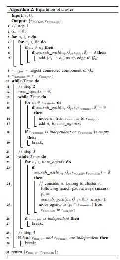
It is noteworthy that during the bipartition process, agents in the remaining set will be moved to the major set. The bipartition of a cluster comprises four steps:
1, identify the maximum unavoidable agents of the cluster, referred to as the major set;
2, examine each agent in the remaining set to determine if its dependence path must pass through agents of the major set. Move agents meeting this criterion to the major set;
3, Check any newly added agents to the major set to ascertain if their dependence paths must pass through agents in the remaining set. Transfer such agents from agents the remaining set to the major set;
4, verify whether the major set and the remaining set both meet the requirements of the cluster. If they do (or if the remaining set is empty), exit and return the major set and the remaining set as the result of the bipartition. Otherwise, proceed to step 2;
The bipartition process of a cluster concludes when both sets satisfy the cluster’s requirements, or when there are no remaining agents, indicating that the cluster cannot be further decomposed into smaller clusters. The pseudocode for bipartitioning a cluster is outlined in Algorithm 2.
C. Decomposing to levels and sorting
Clusters can be solved irrespective of the order of solving, thus providing an opportunity to decompose MAPF into smaller problems by considering the order of solving. By considering the order of solving, we can divide two agents into different subproblems even if one agent’s dependence path
contains the start or target of another agent. We refer to these smaller problems decomposed from clusters as levels. In this section, we focus on how to decompose clusters into levels and determine the order of solving. To facilitate this discussion, we introduce some new concepts.
Definition 10: Order of solving agents: If an agent ai must be solved before another agent aj , we denote it as ai > aj ; if ai must be solved later than aj , we denote it as ai < aj . It is important to note that both ai > aj and ai < aj can coexist (indicating that both agents must be solved in the same problem) or neither can exist (indicating no order limitation between solving ai and aj ).
The order of solving agents is determined by whether an agent’s dependence path contains another agent’s start or target. If ai’s dependence path contains aj ’s start, it implies that ai must be solved later than aj to ensure that aj ’s start is not occupied. Conversely, if ai’s dependence path contains aj ’s target, ai must be solved before aj to ensure that aj ’s target is not occupied. Furthermore, the order of solving levels is determined by the order of solving agents within them.
Definition 11: Solving order graph Gs of a cluster: a directed graph representing whether an agent must be solved before another agent. Its nodes are agents, and edges indicate the order of solving between agents. The structure of the solving order graph is determined by each agent’s dependence path. Specifically, if agent ai must be solved before agent aj , the corresponding edge in Gs is denoted as ai → aj .
Definition 12: Level: a level is a strongly connected component of Gs. Intuitively, a level is a group of agents that form a loop in Gs, indicating that the agents within the loop must be solved simultaneously. For example, if three agents A, B, and C are in the same loop such that A → B → C → A, it implies that A must be solved before B, B before C, and C before A. Thus, A, B, and C can only be solved simultaneously. Unlike clusters, where the order of solving is arbitrary, the order of solving levels is determined. The order of solve levels is determine by the edge in Gs that connect them. The order of solving levels is determined by the edges in Gs that connect them.
Definition 13: Order of solving levels: if a level li must be solved before another level lj , we denote it as li > lj ; if li must be solved later than lj , we denote it as li < lj .
Definition 14: Level ordering graph Gl is a directed graph whose nodes are levels, and edges indicate whether a level must be solved earlier than another level. If there is no edge connecting two levels, this implies that there is no explicit order to solve them, although there may be an implicit order.
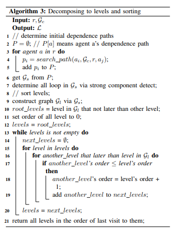
For example, if level A has no edge connecting to level C, but level A is connected to level B and level B is connected to level C, it implies that level A must be solved earlier than level C. Essentially, Gl serves as a condensed version of Gs. There are five steps involved in decomposing a cluster into multiple levels and determining the order of solving: 1, determine each agent’s dependence path, and available agents constrained to the agents of the current cluster; 2, obtain the solving order graph Gs from the dependence paths of the current cluster; 3, identify all strong components of Gs as levels; 4, determine the relationships between levels by examining the edges that connect them.
Construct the level ordering graph Gl , which represents the order of solving between levels. 5, set levels that are not later than any other levels as root levels. Then, using Breadth First Search, traverse all levels in Gl , where the order of the last visit to each level represents the order of solving them; In implementation, Tarjan’s algorithm [19] is utilized to determine strongly connected components from a directed graph. It is important to note that after completing all steps of decomposition, we ensure that the final subproblems do not compromise solvability.
The entire process of decomposing into levels and sorting them is depicted in Algorithm 3. However, we cannot guarantee that the final subproblem is the optimal decomposition. Analogous to using gradient descent to solve non-linear optimization problems, we progressively get smaller and smaller subproblems, but the final result may still not be the global optimal solution.
D. Solving and combining
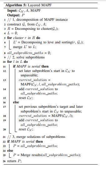
After completing the decomposition of a MAPF instance, the next step involves considering how to solve the subproblems separately and combine their results without conflicts. There are two main types of MAPF methods: serial MAPF methods and parallel MAPF methods. Serial MAPF methods, such as CBS-based methods, can use external paths as constraints to avoid conflicts, as they search for an agent’s path while the paths of other agents remain static. On the other hand, parallel MAPF methods, such as LaCAM and PIBT, cannot always treat external paths as dynamic obstacles to avoid, as they may avoid the same state (all agents’ locations) occur multiple times. For simplicity in this article, we do not set external paths as dynamic obstacles to avoid for all parallel MAPF methods.
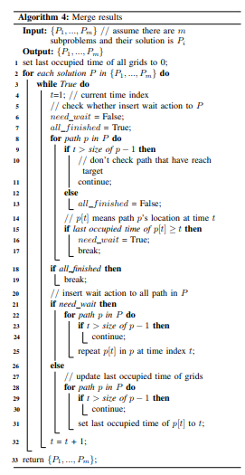
In serial MAPF methods, we only need to merge separate results into a single set. However, for the second type of MAPF method, we need to add wait actions in the resulting paths to avoid conflicts between paths from different subproblems, as shown in Algorithm 4. In the following, we define serial MAPF as MAPF(CN , A, P), and parallel MAPF methods as MAPF(CN , A), where A represents agents and P represents external paths that need to be avoided.
The overall process of decomposing a MAPF instance into multiple subproblems, solving the subproblems, and merging their results is illustrated in Algorithm 5. As mentioned earlier, our decomposition method ensures the solvability of subproblems by ensuring the existence of a solution under the simplified scenario. However, our method does not guarantee that we find the optimal decomposition. While we have not provided theoretical analysis regarding this issue in this manuscript, we offer empirical analysis based on extensive testing, as detailed in Section VI.
Authors:
- Zhuo Yao
- Wei Wang
This paper is
[story continues]
tags