A Smarter Way to Scale Multi-Agent Pathfinding

Table Of Links

ABSTRACT

I. INTRODUCTION

II. RELATED WORKS

III. PRELIMINARIES

IV. METHODOLOGY

V. RESULTS OF DECOMPOSITION

VI. RESULTS OF DECOMPOSITION’S APPLICATION

VII. CONCLUSION, ACKNOWLEDGMENTS AND REFERENCES

III. PRELIMINARIES

A. Basic definitions

In this section, we present fundamental definitions of multi-agent pathfinding. Since our method is dimensionindependent, the provided definitions apply to any-dimensional grid space CN .

1. Grid space: Let CN (N ≥ 2) denote a finite N -dimensional integer Euclidean space, where the size of the space is defined as D → CN , with D = {d1, d2, . . . , di , . . . , dN } and di ∈ N. The coordinates of an element g in this space are defined as a vector (x1, x2, . . . , xi , . . . , xN ), where xi ∈ ([0, di) ∩ N).
2. Grid states: There are only two possible states for a grid/element in CN : passable or unpassable. The set of all passable grids in CN is denoted as F → CN , while the set of all unpassable grids is denoted as O → CN . Therefore, (F → CN )∪(O → CN ) = CN , (F → CN )∩(O → CN ) = ∅. For convenience, we denote all grids outside of CN as unpassable. If a path passes no unpassable grids, we denote it as collision-free; otherwise, it collides with obstacles.
3. Neighborhood of grid: Denote δ(g) as the neighborhood of grid g, which consists of the closest 2N grids near g.
4. Agents: Assuming there are k agents A = {a1, a2, . . . , ak} in the grid space CN , where each agent always occupies a passable grid. Their starting grids are denoted by S = {s1, s2, . . . , sk}, and their target grids are denoted by T = {t1, t2, . . . , tk}. Each agent has a unique starting grid and a targeting grid. Specifically, for all i ∈ {1, 2, . . . , k} and j ∈ {1, 2, . . . , k} with i ̸= j, we have si ̸= sj , ti ̸= tj , si ̸= tj , and ti ̸= sj .
5. Time stamp: Time is discretized into timesteps. At each timestep, every agent can either move to an adjacent grid or wait at its current grid.
6. Path: A path pi for agent ai is a sequence of grids that are pairwise adjacent or identical (indicating a wait action), starting at the start grid si and ending at the target grid ti . The cost of a path is the number of time steps it takes, i.e., the size of the path sequence |pi |. We assume that the agents remain at their targets forever after completing their paths.
7. Conflict: We say that two agents have a conflict if they are at the same grid or exchange their positions at the same timestep.
8. Solution: A solution of a MAPF instance is a set of conflict-free paths {p1, p2, . . . , pk}, one for each agent. Generally, an optimal solution is one with minimal sum of costs (SOC) Pk i=1 |pi | or makespan argmax i∈{1,2,...,k} |pi |. In this manuscript, we consider the effects of decomposition on both SOC and makespan.
9. Solvability: If there exists a solution for a MAPF instance, it is solvable. In the manuscript, we only consider the decomposition of solvable MAPF instances. A MAPF method is considered complete if it can always find a solution for a solvable problem; otherwise, it is incomplete. For example, EECBS is complete while PBS is incomplete. A method to determine whether a MAPF instance is solvable is whether every agent can find a collision-free path (i.e., pass no unpassable grids) from the grid space. It is noteworthy that passing through other agents’ starting or target grids is acceptable.

Decomposition of MAPF instance: Considering that the cost of solving a MAPF instance grows nearly exponentially as the number of agents increases [7], decomposing a MAPF instance and solving subproblems typically incurs lower costs compared to solving the raw instance.

To reduce the cost of solve MAPF instance, we proposed a new technique: splitting a MAPF instance with multiple agents into multiple subproblems, each with fewer agents but under the same map, and solving these subproblems in a specific order. Here, we define the number of agents in each subproblem as the size of the subproblem. When solving a subproblem, it is crucial to ensure that the current paths do not conflict with the paths from previous subproblems. If every subproblem is solvable, combining all subproblems’ results yields the solution of the original MAPF instance.

The criteria for judging whether one decomposition is better than another involves sorting the subproblems’ sizes in decreasing order and comparing the sizes of the subproblems from the largest to the smallest. The first smaller subproblem encountered indicates the better decomposition.

For example, suppose there are two decompositions of a MAPF instance with 100 agents. The sizes of the subproblems for the first decomposition are 40, 20, 15, 14, and 11, while for the second decomposition, they are 40, 20, 19, 13, and 8. The first decomposition is considered better than the second one because the third cluster’s size (15) in the first decomposition is smaller than the second decomposition’s third subproblem size (19).

We compare the quality of decomposition in this manner because the cost of solving a MAPF instance grows exponentially as the number of agents increases [7]. In theory, solving all agents together has a higher chance of finding a shorter solution compared to solving them separately. Therefore, MAPF methods with decomposition of MAPF instances tend to produce worse solutions than raw methods. However, we provide no theoretical analysis regarding the extent of this degradation in this manuscript; hence, we conduct empirical comparisons through extensive testing in Section VI.

In implementation, we measure the quality of decomposition by calculating the ratio between the size of the maximum subproblem and the number of agents of the raw MAPF instance. Since the cost of solving a MAPF instance is mainly determined by the maximum subproblem’s size, we refer to such a ratio as the decomposition rate in the following text.

Based on the criteria for comparing decompositions, a MAPF instance has a certain optimal decomposition that is better than all other decompositions. We have not found a direct way to obtain the optimal decomposition, but we can optimize an initial decomposition progressively to achieve a better decomposition.

B. Theory basis of decomposition

A decomposition of a MAPF instance is considered legal if each subproblem remains solvable. Before discussing how to decompose a MAPF instance, we introduce how to check whether a decomposition of a MAPF instance is legal, i.e., every subproblem should have a solution that avoids conflicts with other subproblems’ paths.

We can simplify this by having each subproblem’s agents move until all previous subproblems have reached their targets, while avoiding the starts of subproblems that haven’t been solved yet. In this simplified scenario, every subproblem only needs to avoid previous subproblems’ targets and later subproblems’ starts. If we can find a solution for a subproblem under this simplified scenario, it is solvable. If we can find such a solution for every subproblem of a decomposition under the simplified scenario, the decomposition does not sacrifice the completeness of MAPF.

We check the solvability of a decomposition by verifying whether every agent of every subproblem can find a path under the simplified scenario. Essentially, the simplified scenario limits each subproblem’s agents to move only within a specific layer of the time-spatial space, where each layer has a unique timestep range. Therefore, we call our method LayeredMAPF. However, it is crucial to note that the solution under the simplified scenario may not be the only conflict-free solution, and the simplified scenario may generate solutions with extra wait actions. Thus, we will set the previous subproblem’s solution as constraints to avoid if a MAPF method supports it (serial MAPF methods). For MAPF methods that do not support setting external paths as constraints (parallel MAPF methods), we will set the previous subproblems’ targets and the later subproblems’ starts as occupied to ensure completeness.

To reduce the time cost of searching for paths, we propose a connectivity graph Gc, whose nodes consist of free grid groups and the starts and targets of agents, and edges represent connectivity between nodes.

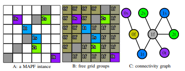
Definition 1: A free grid group is defined as a set of passable grids that contains no start or target grid of agents, and there always exists a path connecting any two grids within the group (where each waypoint in the path is within the same free grid group). We denote a free grid group as fg and a set of free grid groups as Fg. An example about free grid group are shown in Fig. 2.

Definition 2: The connectivity graph Gc is an undirected graph whose nodes consist of free grid groups, starting points, and targets for all agents, with edges representing the connectivity between these nodes.

Definition 3: The dependence path of an agent ai is defined as the path from si to ti , consisting of nodes in Gc. As an example, the dependence path for agent 0 in the instance shown in Fig. 2 is ”0s → 0f → 1t → 1f → 0t”; for agent 1, it is ”1s → 1f → 1t”; and for agent 2, it is ”2s → 1f → 2t”

The dependence path of an agent reflects its relationship with other agents. For a valid decomposition, each agent’s path must not intersect with the targets of previous subproblems or the starts of later subproblems. The dependence paths of agents determine whether two agents must be solved in the same subproblem or the order in which they are solved across different subproblems. Specifically, there are four cases:

1, if the dependence path of agent ai contains only the start of agent aj , it indicates that ai should be solved after aj ;

2, if the dependence path of agent ai contains only the target of agent aj , it implies that ai should be solved before aj ;

3, if the dependence path of agent ai contains both the start and target of agent aj , it signifies that ai and aj must be solved in the same subproblem;

4, if the dependence path of agent ai contains neither the start nor the target of agent aj , it suggests that ai and aj can be solved in different subproblems, and the order of solving them does not matter.

It is worth noting that an agent’s dependence path is not unique. By updating their dependence paths, we can alter the relationship between two agents (in implementation, we check for the existence of such paths rather than explicitly maintaining all agents’ dependence paths). By changing the relationship between two agents, we can update the subproblems of a Multi-Agent Path Finding (MAPF) instance’s decomposition. Although there is no direct method to ensure that agents’ dependence paths correspond to smaller subproblems, we have proposed several approaches to encourage the generation of smaller subproblems; their details can be found in Section IV.

Here, we define the function for searching dependence paths as pi = search path(ai , Gc, available nodes, avoid nodes). Here, Gc represents the connectivity graph of the MAPF instance, available nodes are those nodes in Gc that can be traversed, and avoid nodes are those nodes that must be avoided.

Specifically, an empty set for available nodes means that all nodes are available. If the search path function succeeds, it returns a path; otherwise, it returns an empty set. If not specified, both available nodes and avoid nodes default to being empty. In detail, the search path function is implemented using a classic Best First Search approach, similar to A*. For this function, the cost and heuristic value represent the number of nodes the path has visited and the number of agents the path will visit. We consider a path to have visited an agent if it contains the start or target of that agent.