
Quantization is a powerful technique widely used in machine learning to reduce the memory footprint and computational requirements of neural networks by converting floating-point numbers into lower-precision integers. This approach helps models run efficiently on embedded devices and edge hardware.
In this article, we'll explore quantization in detail, implementing a simple quantization and dequantization process from scratch, and demonstrate how to use it within PyTorch models.
What is Quantization?
Quantization of Neural Networks is the process of converting the weights and activations of a neural network from high-precision formats (typically 32-bit floating-point numbers, or float32) to lower-precision formats (such as 8-bit integers, or int8).
The main idea behind quantization is to “compress” the range of possible values in order to reduce data size and speed up computations.
Neural networks are becoming larger and more complex, but their applications increasingly require running on resource-constrained devices such as smartphones, wearables, microcontrollers, and edge devices. Quantization enables:
- Reducing model size: For example, switching from float32 to int8 can shrink a model by up to 4 times.
- Faster inference: Integer arithmetic is faster and more energy-efficient.
- Lower memory and bandwidth requirements: This is critical for edge/IoT devices and embedded scenarios.
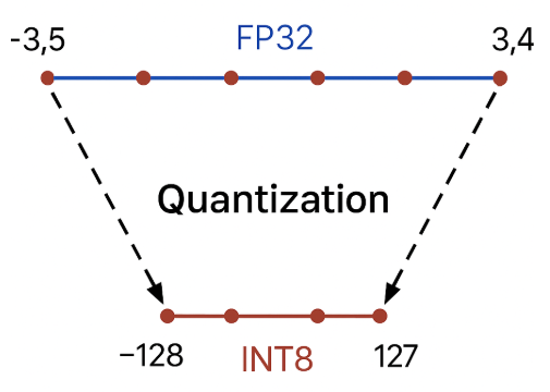
During quantization, the values of weights and activations are mapped from their original continuous range to discrete levels using simple linear transformations.
For example, the range of values [-3.5, 3.4] can be “sliced” into 256 levels (int8), and each real value is rounded to the nearest discrete level.
In neural networks, quantization most commonly refers to converting two types of data: weights and activations.
- Weights are the parameters that the network “remembers” during training. They determine how strongly each input affects the output of a neuron. Quantizing the weights can significantly reduce the overall model size, since weights typically take up most of the memory.
- Activations are the values computed at the output of each layer during the network’s operation (inference). Essentially, these are the signals “passed” from one layer to the next. Quantizing the activations is important for speeding up inference because most operations inside the neural network are performed on activations.
Asymmetric and Symmetric Quantization
When we quantize values, we need to “compress” the original range of numbers and correctly map them between float and int.
This is achieved using two key parameters scale - a coefficient that indicates how much one step in the integer representation corresponds to a change in the float value, and zero_point - an integer value that specifies which int8 value corresponds to zero in the float representation.
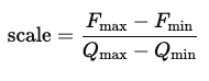
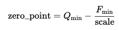
whereFmax, Fmin- the maximum and minimum float valuesQmax, Qmin - the maximum and minimum integer values (127 and -128 for int8)
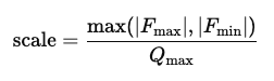
There are two main approaches: symmetric and asymmetric quantization. The main difference between symmetric and asymmetric quantization lies in how they map the ranges of original float values to quantized integers. With symmetric quantization, the float value range is always centered around zero (zero_point is 0), so zero in the float domain corresponds to zero in the integer representation.
This simplifies calculations and speeds up inference, but requires the values to be distributed roughly equally on both the positive and negative sides.
In contrast, asymmetric quantization can work with any range, not necessarily symmetric, and allows you to shift “zero” to the appropriate point. This is achieved using a zero point, which defines which integer value corresponds to zero in the float range. This approach is especially convenient when all the values in a tensor are positive or have a non-standard range, for example, after applying a ReLU activation.
In modern neural networks, weights are most often quantized symmetrically, while activations are quantized asymmetrically, to achieve the best balance of accuracy and performance on real devices.
The formulas for quantization and dequantization are as follows:
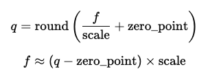
where
f - the original float value
q - the quantized value
Implementing Asymmetric Quantization in PyTorch
This example demonstrates how to manually implement asymmetric quantization and dequantization of a tensor using PyTorch.
First, a random tensor with float32 values is generated
import torch

# Generate a random 2D FP32 tensor (e.g., 4x5)
x_fp32 = torch.randn(4, 5) * 5
print("Original FP32 tensor:\n", x_fp32)
Then, the minimum and maximum values of this tensor are computed, and these are used to calculate the parameters scale and zero_point for asymmetric quantization
# Find min/max for the whole tensor
x_min, x_max = x_fp32.min(), x_fp32.max()

qinfo = torch.iinfo(torch.int8)
qmin, qmax = qinfo.min, qinfo.max

# Calculate scale and zero_point for asymmetric quantization
scale = (x_max - x_min) / (qmax - qmin)
zero_point = int(torch.round(qmin - x_min / scale))
Next, the tensor is converted to the integer format int8, and the values are rounded, scaled, and shifted to fit into the valid int8 range.
# Quantize to INT8
x_q = torch.clamp(torch.round(x_fp32 / scale + zero_point), qmin, qmax).to(torch.int8)
print("\nQuantized INT8 tensor:\n", x_q)
For testing purposes, the quantized values are transformed back to the original float32 range using the inverse formula.
# Dequantize back to FP32
x_dequant = (x_q.float() - zero_point) * scale
print("\nDequantized FP32 tensor:\n", x_dequant)
Finally, quantization errors are calculated -mean squared error (MSE) and the maximum absolute error between the original and restored tensors.
# Compare: MSE and max absolute error
mse = torch.mean((x_fp32 - x_dequant) ** 2)
max_abs_err = (x_fp32 - x_dequant).abs().max()
print(f"\nMSE between original and dequantized: {mse:.6f}")
print(f"Max absolute error: {max_abs_err:.6f}")
This example clearly illustrates how the main steps of asymmetric quantization work in practice, and what kinds of distortions can occur when converting between float and integer representations.
Below is the output from running the code:
Original FP32 tensor:
 tensor([[ 2.8725,  1.0017, -4.8329, -0.8561,  2.7119],
        [ 9.3110, -2.9099, -9.1575,  7.8362,  4.5481],
        [-2.4224,  6.4360,  1.0812, -8.9195,  7.3958],
        [-1.5830, -1.7517,  4.6271, -9.3345, -9.3382]])

Quantized INT8 tensor:
 tensor([[  39,   14,  -66,  -12,   37],
        [ 127,  -40, -125,  107,   62],
        [ -33,   88,   15, -122,  101],
        [ -22,  -24,   63, -128, -128]], dtype=torch.int8)

Dequantized FP32 tensor:
 tensor([[ 2.8522,  1.0239, -4.8268, -0.8776,  2.7060],
        [ 9.2880, -2.9254, -9.1417,  7.8253,  4.5343],
        [-2.4134,  6.4358,  1.0970, -8.9223,  7.3865],
        [-1.6089, -1.7552,  4.6074, -9.3611, -9.3611]])

MSE between original and dequantized: 0.000275
Max absolute error: 0.026650
As you can see from the calculated metrics, the error between the quantized and the original tensor is very small and, in most cases, negligible for practical tasks.
Post-Training Symmetric Quantization of a Linear Layer
In this section, we implement and test a simple linear layer with post-training symmetric quantization.
ThePTQSymmetricQuantizedLinear class extends nn.Module and mimics a standard fully-connected layer, but adds the ability to quantize its weights after training using 8-bit symmetric quantization.
After training, we can call the quantize_weights() method, which converts the learned float32 weights into quantized int8 values and stores the corresponding scale. During inference (forward), the layer reconstructs the original weights from their quantized representation and computes the output as usual.
import torch
import torch.nn as nn
import torch.nn.functional as F

class PTQSymmetricQuantizedLinear(nn.Module):
    def __init__(self, in_features, out_features, bias=True):
        super().__init__()
        self.in_features = in_features
        self.out_features = out_features

        self.weight = nn.Parameter(torch.empty(out_features, in_features))
        if bias:
            self.bias = nn.Parameter(torch.empty(out_features))
        else:
            self.register_parameter('bias', None)

        # buffers for storing quantized weights and scale
        self.register_buffer('weight_q', None)
        self.register_buffer('weight_scale', None)

    @staticmethod
    def symmetric_quantize(x):
        qmax = 127
        max_abs = x.abs().max()
        scale = max_abs / qmax if max_abs > 0 else 1.0
        x_q = torch.round(x / scale).clamp(-qmax, qmax)
        return x_q.to(torch.int8), torch.tensor(scale, dtype=torch.float32, device=x.device)

    def quantize_weights(self):
        w_q, w_scale = self.symmetric_quantize(self.weight.data)
        self.weight_q = w_q
        self.weight_scale = w_scale

    def forward(self, input):
        weight_deq = self.weight_q.float() * self.weight_scale
        return F.linear(input, weight_deq, self.bias)
Below, we show how to initialize the layer, quantize the weights, run inference, and compare the quantized result to the original float32 output. This workflow clearly demonstrates that symmetric quantization can significantly compress the model while preserving most of its numerical accuracy.
layer = PTQSymmetricQuantizedLinear(in_features=4, out_features=3)

# Initialize weights and bias for reproducibility
torch.manual_seed(0)
nn.init.uniform_(layer.weight, -1, 1)
nn.init.uniform_(layer.bias, -0.1, 0.1)

# Generate dummy input
x = torch.randn(2, 4)  # batch_size=2, in_features=4

# Quantize weights
layer.quantize_weights()

# Run forward pass
out = layer(x)
print("Output after quantization:", out)

# Compute the float32 (original) layer output
with torch.no_grad():
    out_fp = F.linear(x, layer.weight, layer.bias)
print("Output original float32:", out_fp)

# Compute the difference (MSE)
mse = torch.mean((out - out_fp) ** 2)
print("MSE between quantized and float32:", mse.item())
Below is the output from running the code:
Output after quantization: tensor([[-0.2760,  0.6149, -0.0378],
        [-1.6489,  1.8015, -0.4852]], grad_fn=<AddmmBackward0>)
Output original float32: tensor([[-0.2753,  0.6172, -0.0395],
        [-1.6417,  1.8051, -0.4910]])
MSE between quantized and float32: 1.781566970748827e-05
Conclusion
Quantization is a key technology that enables modern neural networks to run not only on powerful servers but also on resource-constrained devices such as smartphones, wearables, microcontrollers, and edge devices. By converting weights and activations from float32 to the more compact int8 format, models become significantly smaller, require less memory and computation, and inference times are noticeably reduced.
In this article, we explored how quantization works, discussed the differences between symmetric and asymmetric approaches, and implemented basic examples of these techniques in PyTorch, from manually quantizing tensors to post-training quantization of neural network layers.
Try It Yourself on GitHub
If you want to explore these examples hands-on, feel free to visit my GitHub repository, where you’ll find all the source files for the code in this article. You can clone the repository, open the code in your favorite IDE or build system, and experiment with it. Enjoy playing around with the examples!
Follow me
[story continues]
tags