Choose the Right Graph Model Faster with HypNF’s Parameter Knobs

Table of Links

Abstract and 1. Introduction

2. Related work

3. HypNF Model

   3.1 HypNF Model

   3.2 The S1/H2 model

   3.3 Assigning labels to nodes

4. HypNF benchmarking framework

5. Experiments

   5.1 Parameter Space

   5.2 Machine learning models

6. Results

7. Conclusion, Acknowledgments and Disclosure of Funding, and References

A. Empirical validation of HypNF

B. Degree distribution and clustering control in HypNF

C. Hyperparameters of the machine learning models

D. Fluctuations in the performance of machine learning models

E. Homophily in the synthetic networks

F. Exploring the parameters’ space

5 Experiments

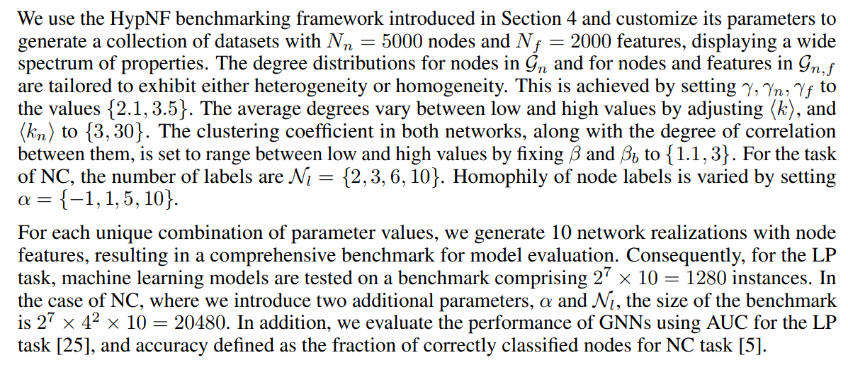
5.1 Parameter Space

5.2 Machine learning models

In this work, we focus on two primary methodologies: feature-based methods, which entail node embedding based on their features, and GNNs, which integrate both features and network topology.

• MLP: A vanilla neural network transforms node feature vectors through linear layers and non-linear activations to learn embeddings in Euclidean space.

• HNN [12]: A variant of MLP that operates in hyperbolic space to capture complex patterns and hierarchical structures.

• GCN [18]: A pioneering model that averages the states of neighboring nodes at each iteration.

• GAT [33]: A model that uses attention mechanisms to assign different importance to different nodes in a neighborhood.

• HGCN [9]: A model that integrates hyperbolic geometry with graph convolutional networks to capture complex structures in graph data more effectively.

Table 2 in Appendix C lists the hyperparameters for training. In the LP task, links are split into training (85%), validation (5%), and test (10%) sets. For the NC task, nodes are distributed as 70%

training, 15% validation, and 15% test [9]. Both tasks follow the methodology in [9], with results averaged over five test-train splits. Models were trained on an NVIDIA GeForce RTX 3080 GPU using Python 3.9, CUDA 11.7, and PyTorch 1.13.

6 Results

We begin by analyzing how topology-feature correlation affects the performance of machine learning models by varying parameters β and βb, which control the coupling between Gn, Gn,f , and the shared metric similarity space. For both NC and LP tasks, Fig. 2 shows that higher topology-feature correlation (β = βb = 3) improves performance for both feature-based and GNN models compared to lower correlation (β = βb = 1.1). In the NC task, feature-based models do not respond to changes in β and perform better with higher βb. Conversely, GNN models, utilizing information from both Gn and Gn,f , benefit from high β and βb values, not only in terms of average performance but also in terms of the spread around this average.

We measured the performance of machine learning models by varying the clustering level in Gn (adjusted by β) and the average number of features per node in the bipartite network, ⟨kn⟩. For the NC task, Fig. 9(a) in Appendix F shows significant performance differences between feature-based and GNN models. In bipartite networks with low ⟨kn⟩, GNN models outperform feature-based ones. As ⟨kn⟩ increases (bottom row), all models’ accuracy improves, converging to almost similar levels. Here, the simplest model, MLP, performs nearly as well as the most sophisticated, HGCN. Note that these results fix β and ⟨kn⟩, averaging over other parameters. Fig. 9(b) in Appendix F compares these models in terms of AUC for the LP task. The models show a significant shift in relative performance with varying ⟨kn⟩. For high ⟨kn⟩, models in hyperbolic space (HNN and HGCN) perform better. Notably, the feature-based model, HNN, matches or exceeds the performance of HGCN, especially at low β.

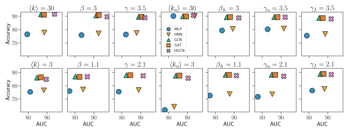
In Fig. 3, we present a summary of model performance on both downstream tasks, varying parameters individually between high and low values while averaging over others. Across most cases, HGCN outperforms or matches others in the LP task, and achieves competitive accuracy in the NC task, akin to other graph-based methods. In addition, for the NC task, the feature-based methods (MLP and HNN) are barely sensible to S 1 model parameters, i.e., ⟨k⟩, β and γ. However, for the LP task, the topology-features correlation strongly impacts their AUC values, leading to MLP and HNN being sensitive to the parameters of the bipartite network, including βb, γn, and γf , with a specific emphasis on ⟨kn⟩. In contrast, GNNs are particularly responsive to variations in ⟨kn⟩. It is worth mentioning that these observations highlight the sensitivity of graph machine learning methods to individual parameters. However, in real-world scenarios, the collective interplay of all parameters influences the overall performance of the models, see the detailed analysis in Appendix F.

Another important factor that is usually overlooked concerns the fluctuations of the performance of machine learning models, which provides insights into their robustness and reliability. We address this problem by analyzing the difference in the standard deviation of the accuracy and AUC for a given set of parameters. In Fig. 7 of Appendix D, we show how the fluctuation changes when each

parameter is set to high or low. Let us take HGCN as an example. For the high average degree ⟨k⟩, the accuracy and AUC display lower standard deviations as compared to low average degree, which means that HGCN is more robust to other parameters when the average degree is high. Moreover, a homogeneous degree distributions (γ = 3.5) results in a broader spread of AUC but not of accuracy. GCN and GAT display similar fluctuation behaviors, whereas for the feature-based models (MLP, HNN), the bipartite-S1 parameters dictate their sensibility to other parameters.

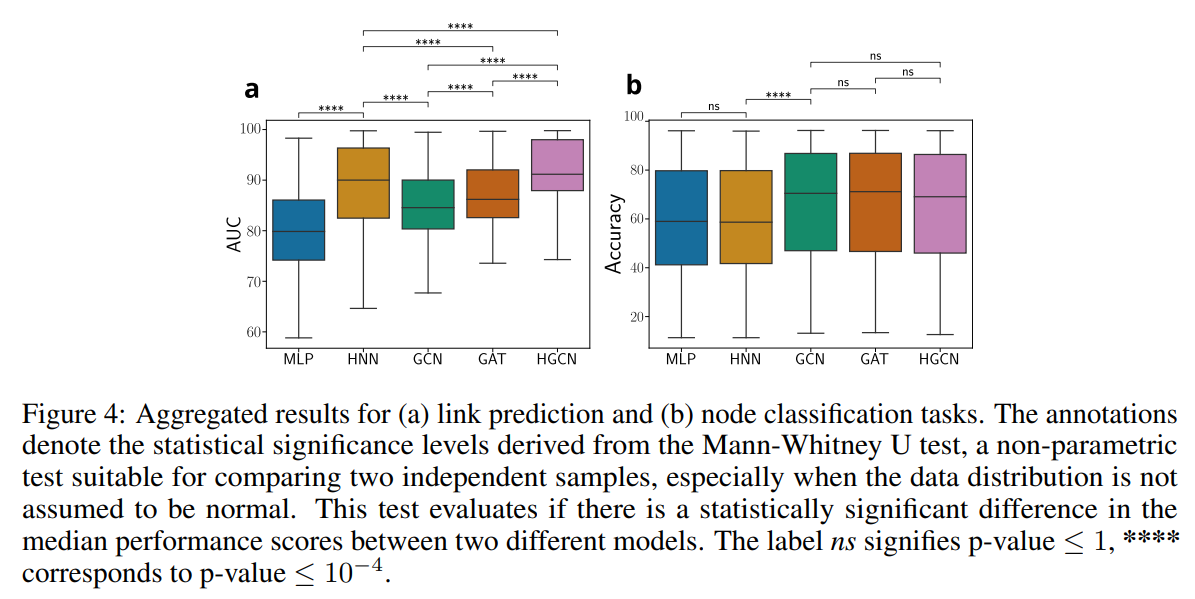
The global average picture of the performance of the analyzed models is shown in Fig. 4, where we averaged results over all the parameters in the HypNF benchmarking framework. This analysis sheds light on model selection when no structural information is available about the data. We observe the superiority of the hyperbolic-based models in capturing essential network properties and connectivities for the LP task (Fig. 4(a)). Yet, HGCN outperforms HNN with statistical significance. As for the NC task, results are more ambiguous, with GNNs outperforming feature-based models overall. However, the distinctions in performance within the GNNs are not substantial. Hence, when dealing with unseen data, the simplicity of the GCN model makes it a more efficient choice.

Finally, in Appendix F, we carry out a comprehensive analysis of the performance of the selected models, focusing on all parameters within the S1/H2 (Figs. 10(a) and 11(a)), bipartite-S1/H2 (Figs. 10(b) and 11(b)), and the combination of the two (Figs. 12 and 13). Moreover, Fig. 14 reveals the dependence of the number of labels and the homophily level in terms of accuracy.