
Table of Links
-
Experiments
C. Technical Details
C.1. Notations
The mathematical notations are described in Table 4.
C.2. Algorithm
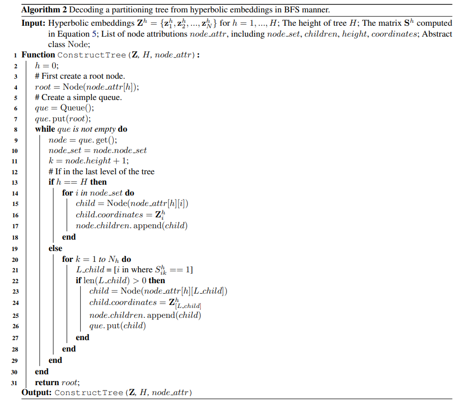
The Algorithm 2 is the decoding algorithm to recover a partitioning tree from hyperbolic embeddings and level-wise assignment matrices. we perform this process in a Breadth First Search manner. As we create a tree node object, we put it into a simple queue. Then we search the next level of the tree nodes and create children nodes according to the level-wise assignment matrices and hyperbolic embeddings. Finally, we add these children nodes to the first item in the queue and put them into the queue. For convenience, we can add some attributes into the tree node objects, such as node height, node number, and so on.
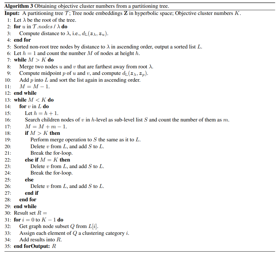
In Algorithm 3, we give the approach to obtain node clusters of a predefined cluster number from a partitioning tree T . The key idea of this algorithm is that we first search the first level of the tree if the number of nodes is more than the predefined numbers, we merge the nodes that are farthest away from the root node, and if the number of nodes is less than the predefined numbers, we search the next level of the tree, split the nodes that closest to the root. As we perform this iteratively, we will finally get the ideal clustering results. The way we merge or split node sets is that: the node far away from the root tends to contain fewer points, and vice versa.
C.3. Datasets & Baselines
We evaluate our model on a variety of datasets, i.e., KarateClub, FootBall, Cora, Citeseer, Amazon-Photo (AMAP), and a larger Computer. All of them are publicly available. We give the statistics of the datasets in Table 1 as follows.
In this paper, we compare with deep graph clustering methods and self-supervised GNNs introduced as follows,
• RGC (Liu et al., 2023a) enables the deep graph clustering algorithms to work without the guidance of the predefined cluster number.
• DinkNet (Liu et al., 2023b) optimizes the clustering distribution via the designed dilation and shrink loss functions in an adversarial manner.
• Congregate (Sun et al., 2023b) approaches geometric graph clustering with the re-weighting contrastive loss in the proposed heterogeneous curvature space.
• GC-Flow (Wang et al., 2023) models the representation space by using Gaussian mixture, leading to an anticipated high quality of node clustering.
• S3GC (Devvrit et al., 2022) introduces a salable contrastive loss in which the nodes are clustered by the idea of walktrap, i.e., random walk trends to trap in a cluster.
• MCGC (Pan & Kang, 2021) learns a new consensus graph by exploring the holistic information among attributes and graphs rather than the initial graph. • DCRN (Liu et al., 2022a) designs the dual correlation reduction strategy to alleviate the representation collapse problem.
• Sublime (Liu et al., 2022b) guides structure optimization by maximizing the agreement between the learned structure and a self-enhanced learning target with contrastive learning.
• gCooL (Li et al., 2022) clusters nodes with a refined modularity and jointly train the cluster centroids with a bi-level contrastive loss.
• FT-VGAE (Mrabah et al., 2022) makes effort to eliminate the feature twist issue in the autoencoder clustering architecture by a solid three-step method.
• ProGCL (Xia et al., 2022) devises two schemes (ProGCL-weight and ProGCLmix) for further improvement of negatives-based GCL methods.
• MVGRL (Hassani & Ahmadi, 2020) contrasts across the multiple views, augmented from the original graph to learn discriminative encodings.
• ARGA (Pan et al., 2018) regulates the graph autoencoder with a novel adversarial mechanism to learn informative node embeddings.
• GRACE (Yang et al., 2017) has multiples nonlinear layers of deep denoise autoencoder with an embedding loss, and is devised to learn the intrinsic distributed representation of sparse noisy contents.
• DEC (Xie et al., 2016) uses stochastic gradient descent (SGD) via backpropagation on a clustering objective to learn the mapping.
• VGAE (Kipf & Welling, 2016) makess use of latent variables and is capable of learning interpretable latent representations for undirected graphs.
C.4. Implementation Notes
LSEnet is implemented upon PyTorch 2.0[3], Geoopt[4], PyG[5] and NetworkX[6]. The dimension of structural information is a hyperparameter, which is equal to the height of partitioning tree. The hyperbolic partitioning tree is learned in a 2−dimensional hyperbolic space of Lorentz model by default. For the training phase, we use Riemannian Adam (Becigneul & Ganea, 2018) and set the learning rate to 0.003.
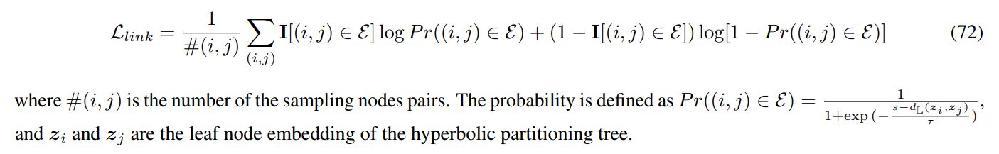
The loss function of LSEnet is the differentiable structural information (DSI) formulated in Sec. 4.2 of our paper. We suggest to pretrain LConv of our model with an auxiliary link prediction loss, given as follows,
Authors:
(1) Li Sun, North China Electric Power University, Beijing 102206, China (ccesunli@ncepu.edu);
(2) Zhenhao Huang, North China Electric Power University, Beijing 102206, China;
(3) Hao Peng, Beihang University, Beijing 100191, China;
(4) Yujie Wang, North China Electric Power University, Beijing 102206, China;
(5) Chunyang Liu, Didi Chuxing, Beijing, China;
(6) Philip S. Yu, University of Illinois at Chicago, IL, USA.
This paper is
[3] https://pytorch.org/
[4] https://geoopt.readthedocs.io/en/latest/index.html
[5] https://pytorch-geometric.readthedocs.io/en/latest/
[6] https://networkx.org/
[story continues]
tags