Exploring Local and Global Sensitivity in Binary Decision Modeling

Table of Links

Abstract and 1. Introduction

2. Basic premises for our models

   2.1. How LLMs are charged

   2.2 An anedotal model from industry

   2.3 Choice of Costs in the Model

   2.4 Why multiple scenarios

3. A Decision Theoretic Model

   3.1 How to model success

4. A Model for Commercial Operations Based on a Single Transaction

   4.1 Example of Using the Model

   4.2 Model Analysis

   4.3 Discussion of the RoI vs. Earning dillema

5. Modelling of a Binary Classification Problem

   5.1 Local Sensitivity Analysis

   5.2 Global Sensitivity Analysis by Sobol Method

6. Related Work

7. Future work

8. Conclusion, References, and Acknowledgements

5 Modelling of a Binary Classification Problem

A binary classification problem is a type of supervised learning task in machine learning where the goal is to predict to which of two classes (categories) a particular instance belongs to [Bishop, 2006]. The output variable in binary classification is typically a categorical variable with two possible values, often represented as 0 and 1, “yes” and “no”, or “true” and “false”.

For example, in a medical diagnosis application, the task might be to classify whether a patient has a particular disease or not based on various input characteristics such as age, blood pressure, cholesterol levels, and other health indicators.

In the context of binary classification, it is crucial to understand the different outcomes that can occur. Usually, the results of binary classification problems are described through a confusion matrix, which lists true positives, false positives, true negatives, and false negatives [Bishop, 2006].

A true positive (TP) occurs when the model correctly predicts the positive class. For example, if the model identifies a transaction as fraudulent and is indeed fraudulent, this is a true positive. In contrast, a true negative (TN) occurs when the model accurately predicts the negative class, such as correctly identifying a non-fraudulent transaction [Bishop, 2006].

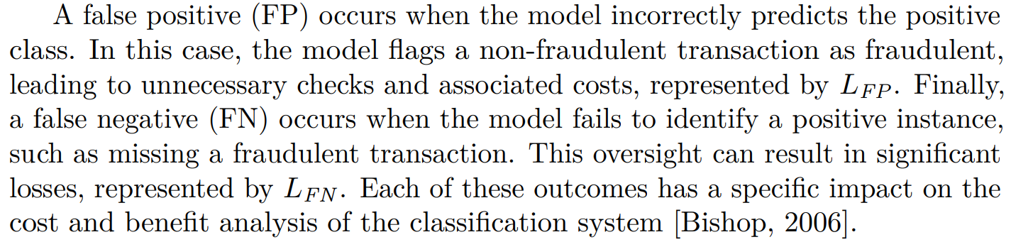
The costs involved with the binary classification operation require a more detailed calculation. First, it must be delimited to what will be done with each operation. Furthermore, considering only the classification as true or false, one must consider the costs related to all possible options between what to do true positives, true negatives, false positives and false negatives.

At first, it is interesting to analyze a change in our representation to consider the different costs.

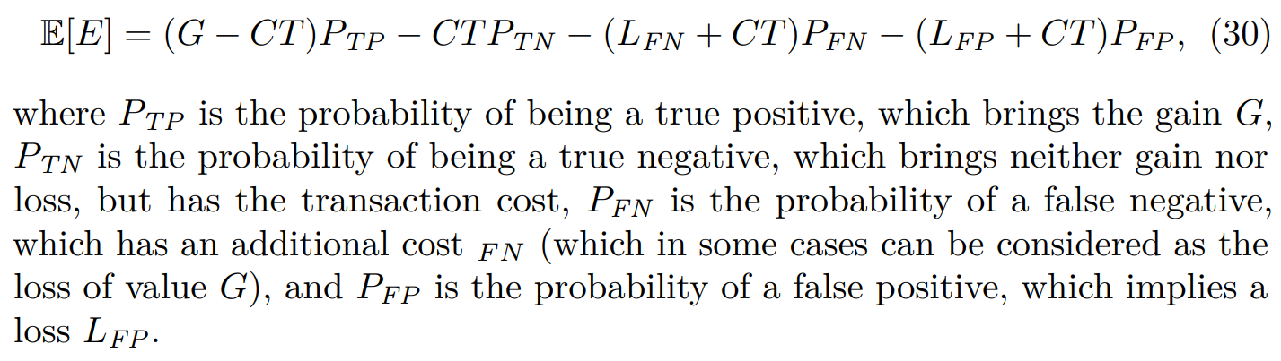
With this modifications, the expected earnings can be modeled as:

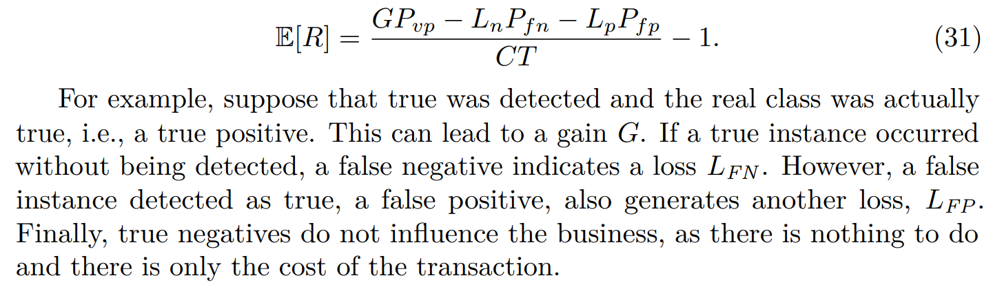
From equation Equation 30 we can calculate RoI as:

5.1 Local Sensitivity Analysis

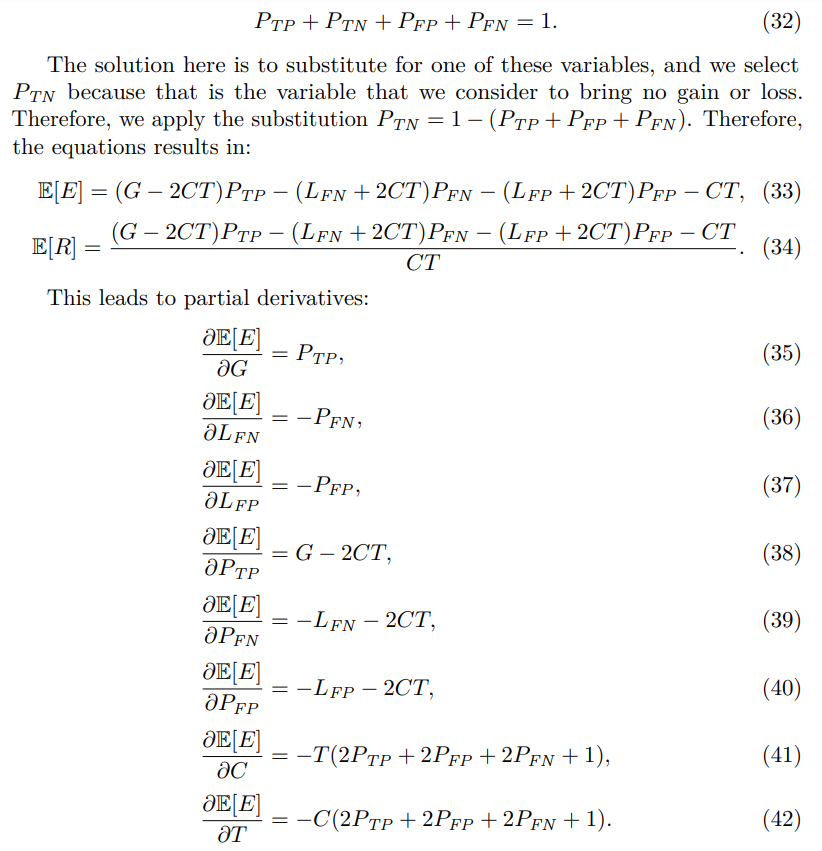
A direct analysis on partial derivatives is not absolutely correct, because there is the restriction that:

Again we checked the Hessian matrix to analyze the linearity and found 48 zeros for 64 partial derivatives E[E], which is fairly linear. However, again the Hessiam matrix for RoI does not show a large number of zeros, so we will skip the local analysis for RoI.

There is a point to note in equations 41 and 42, since they can be rewriten as:

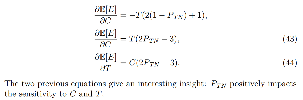
From those previous equations, we see now the separation of influences: while when we used only P and (1 − P) as measures of success and failures, there was a strong interaction between P and G + L. Now there is a separation, G and the different L are mostly influenced by their own probabilities of happening, although there is always the Equation 32 to show interactions among the probabilities.

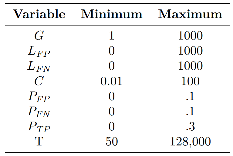
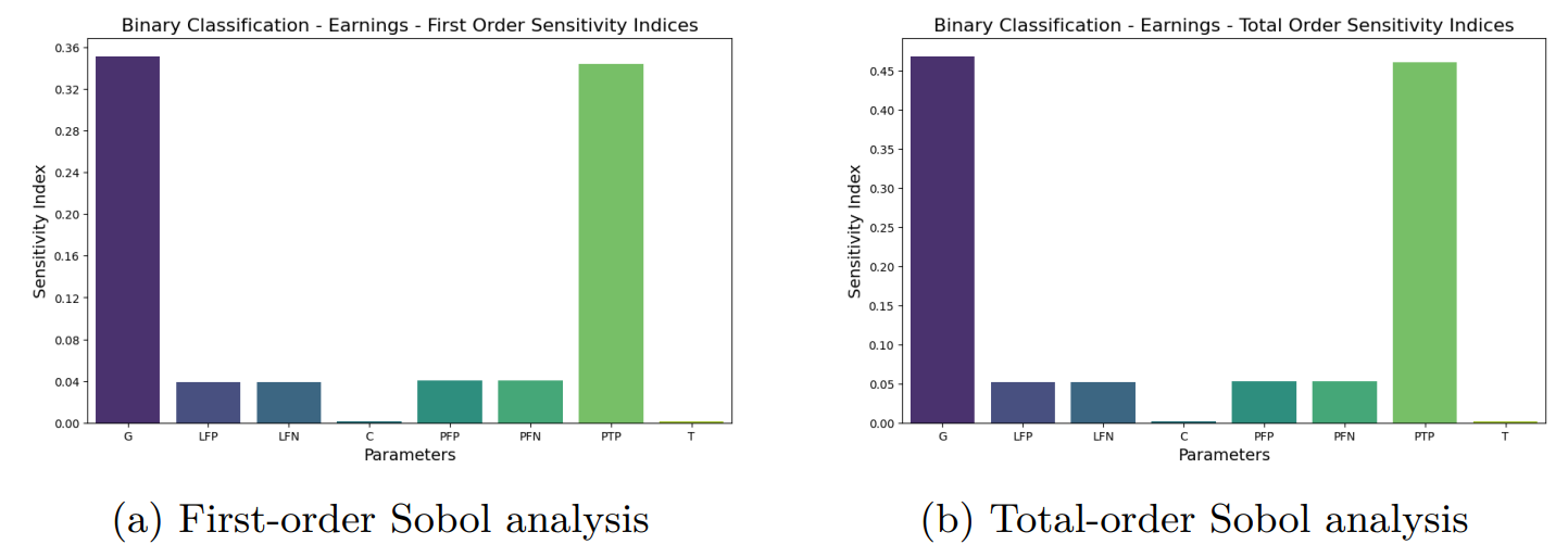
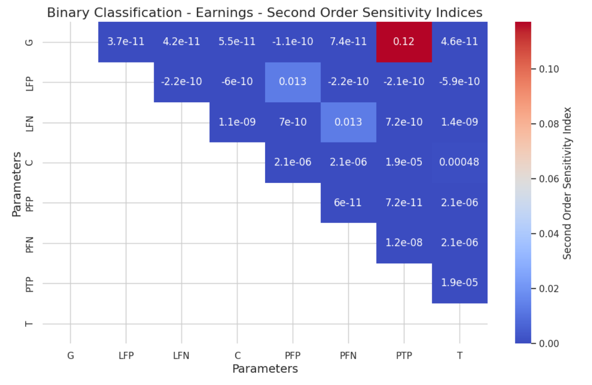
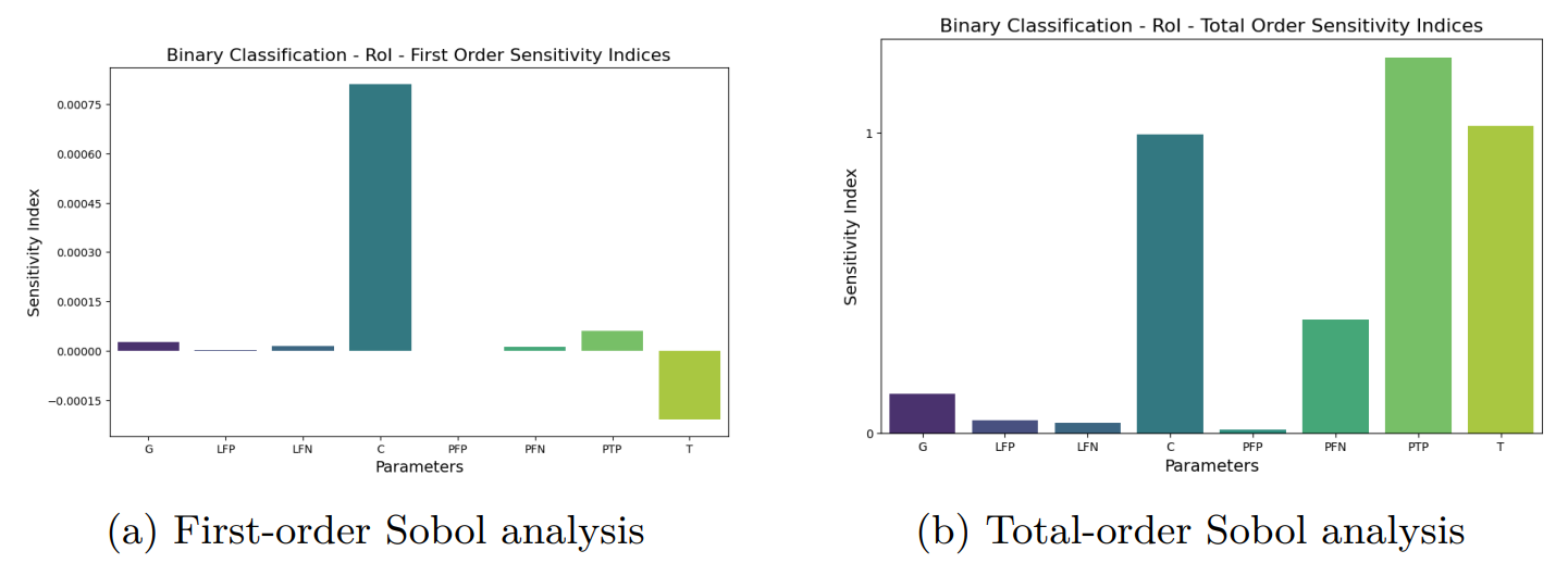
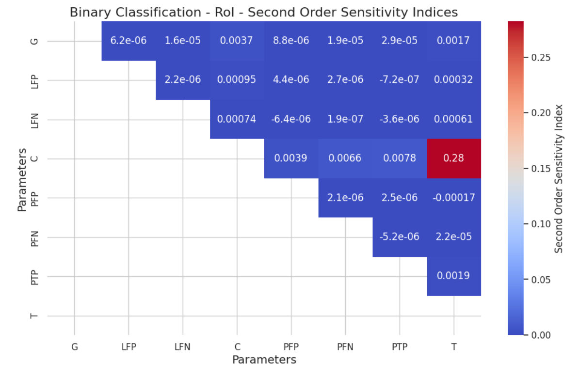
5.2 Global Sensitivity Analysis by Sobol Method