How Public Balance Sheet Data Can Be Used to Estimate Life Insurance Guarantee Costs

Table of Links

1. Introduction
2. Mean-field Libor market model
3. Life insurance with profit participation
4. Numerical ALM modeling
5. Phenomenological assumptions and numerical evidence
6. Estimation of future discretionary benefits
7. Application to publicly available reporting data
8. Conclusions
9. Declarations
10. References

Application to publicly available reporting data

The purpose of this section is to apply the estimation formulae (5.58) and (5.59) for lower and upper bound to publicly available data from a real life insurer (Allianz Lebensversicherung AG in Germany), and to compare the results to the value, F DBCO, that has been derived by the company. In Section 6.1 we collect the necessary data, the estimates and a discussion are then provided in Section 6.2. These estimations are carried out for the accounting years 2017-2022, and are therefore subject to quite different circumstances: low interest rate environment and positive unrealized gains for 2017-2022, and medium-high yield curve in 2022 accompanied by negative unrealized gains.

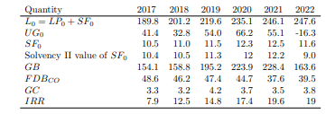
6.1. Allianz Lebensversicherungs-AG: publicly reported values. Formulae (5.58) and (5.59) hinge on the knowledge of specific balance sheet items. These items are contained in publicly available data, and provided for further reference in Table 3. The respective sources are listed in Table 4. The local GAAP value, L0, of life insurance with profit participation is adjusted due to a necessary regrouping of business. This step is explained respectively on the first of the two cited page numbers of the SCR report [36] for each accounting year. The value of UG0 is scaled to L0, which is in line with the general assumption (3.41). The reason behind this scaling is that according to [30, § 3] only the fraction of the capital gains, corresponding to the assets scaled to cover the average value of liabilities in the accounting year under consideration, contribute to the gross surplus. Moreover, the value GB that is used to calculate F DB0 is augmented by the going concern reserve GC. This is because this reserve is a cash-flow that leaves the model (as explained in the quoted source in Table 4) but this cash-flow is not accounted for in our no-leakage principle 2.31, and we do not know to which cash-flow in the comprehensive list recorded in the delegated act [33, Article 28] this going concern reserve should be attributed to.

The relevant risk free rate providing the deterministic discount factors P(0, t) and the initial forwards F 0 t is published by EIOPA at [35]. All other data, for instance technical interest rate and technical gains rate, are as in [14, Section 6]. In particular, the policyholder fraction of the positive gross surplus is gph = 75.5 %.

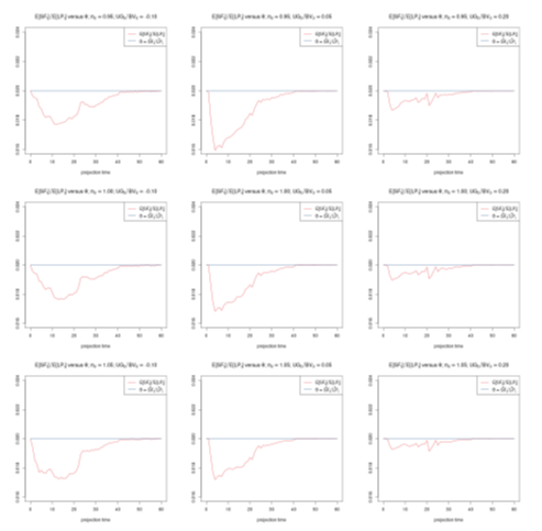
6.2. Estimation. The estimation formulae (5.58) and (5.59) have been implemented in R, and evaluated on the data of Section 6.1. The results of this implementation are displayed in Table 5. 1 The estimations in Table 5 are subject to considerable uncertainty. In [14] we have studied sensitivities of the formulas (5.58) and (5.59) with respect to parameter choices concerning, e.g., technical interest rate, technical gains, or market implied volatility. It was observed that these sensitivities impact the estimation only marginally. This is due to the fact that F DB \is determined to a large extent already by F DB0. However, F DB0 also carries estimation uncertainty, although this may not be obvious at first sight. Indeed, in principle all the data needed to calculate F DB0 are contained in Table 3, apart from gph. In theory these objects are all clearly defined, but in practice we had to: adjust L0 to reflect only life insurance with profit participation, rescale UG0 to L0, increase GB by GC, and deduct SF0 from F DB \. These adjustments were in order so that all items can be interpreted correctly. However, due to incomplete information we cannot know if these were all the necessary adjustments. For example, it may be possible that the regrouping that leads to a rescaling of L0 should also have induced a rescaling of SF0, followed by an appropriate scaling of UG0. The point here is that the calculation of F DB0 is only seemingly trivial but involves in practice a lot of information about the various positions.

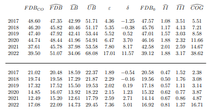
It can be seen that the estimation is successful, i.e. |δ| < ε, in all years, except for one year. In 2021 we observe that F DBCO is slightly smaller than LBd. The cause for this aberration in 2021 cannot be determined from the available data, clearly it may be due to parameter uncertainty as mentioned above. Nevertheless, given that the information that is used to derive Table 5, it is quite remarkable that the estimation error δ is smaller than 3 % MV0 in all cases but 2022. In 2022 it seems that the cost of guarantee term COG \is over-estimated. Apart from the case 2022, the values of δ and ε relative to MV0 are of a similar magnitude as in the numerical study summarized in Table 2.

Even in 2022 we can stipulate a connection between the results in Table 2 and in 5: this year is characterized by negative unrealized gains, UG0, which in Table 2 corresponds to the columns headed by UG0/BV0 = −0.10, and these are the columns with the highest ε values (possibly due to an over-estimation of COG \). It is interesting to compare 2022 to the previous years. This year is associated with a steep rise in interest rate yield, and this caused the unrealized gains, UG0, to become negative. Thus the rise in cost of guarantees is to be expected. Comparing the results in Table 5 to those of 2 (for the columns UG0/BV0) it is plausible that the Monte Carlo algorithm and the management rules used to calculate F DBCO are much more efficient in avoiding guarantee costs than reflected in our formula (5.53) for COG \. This explains the comparatively higher value of δ in 2022, however the estimation result is still successful since |δ| < ε.