Table of Links
-
Harnessing Block-Based PC Parallelization
4.1. Fully Connected Sum Layers
4.2. Generalizing To Practical Sum Layers
-
Conclusion, Acknowledgements, Impact Statement, and References
B. Additional Technical Details
A. Algorithm Details
In this section, we provide additional details of the design of PyJuice. Specifically, we introduce the layer partitioning algorithm that divides a layer into groups of node blocks with a similar number of children in Appendix A.1, and describe the details of the backpropagation algorithm in Appendix A.2.
A.1. The Layer Partitioning Algorithm

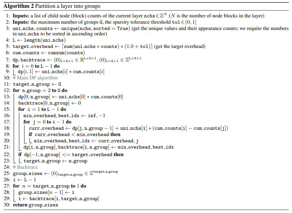

The algorithm is shown in Algorithm 2. A practical trick to speed it up is to coalesce the identical values in nchs as done in line 3. Lines 7-9 initialize the buffers, and lines 11-23 are the main loop of the DP algorithm. Finally, the result partitioning is retrieved using lines 25-29.
Theoretical guarantee. Algorithm 2 is guaranteed to find an optimal grouping given a pre-specified number of groups, and is fairly efficient in practice. We formally state the problem in the following and provide the proof and analysis as follows.
As described in Appendix A.1, the grouping algorithm essentially takes as input a list of “# child node blocks” for each parent node block in a layer, and the goal is to partition all parent node blocks into K groups such that we minimize the following cost: the sum of the cost of each group, where the cost of a group is the maximum “# child node blocks” in the group times the number of parent node blocks in the group. In the following, we first demonstrate that the proposed dynamic programming (DP) algorithm (Algorithm 2) can retain the optimal cost for every K. We then proceed to analyze the time and space complexity of the algorithm.

A.2. Details of the Backpropagation Algorithm for Sum Layers
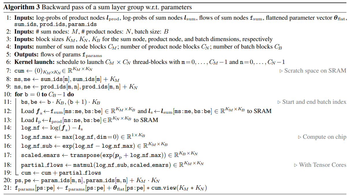
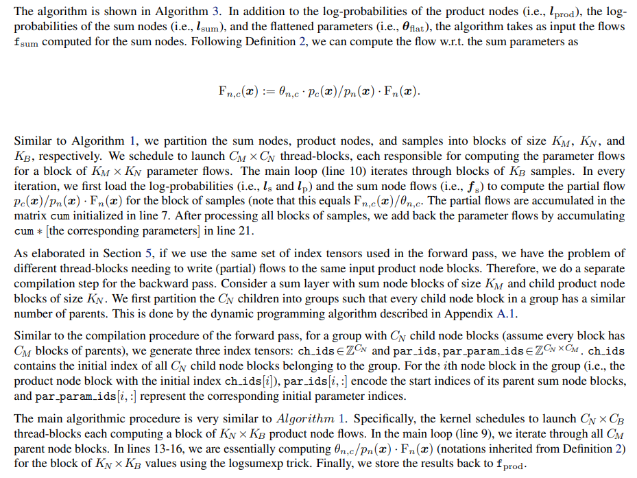
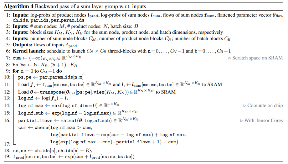
We compute the backward pass with respect to the inputs and the parameters of the sum layer in two different kernels as we need two different layer partitioning strategies to improve efficiency. In the following, we first introduce the backpropagation algorithm for the parameters since it reuses the index tensors compiled for the forward pass (i.e., sum ids, prod ids, and param ids).
A.3. PCs with Tied Parameters
Formally, PCs with tied parameters are PCs containing same sub-structures in different parts of its DAG. Although the nodes in these sub-structures could have different semantics, they can have shared/tied parameters. For example, in homogeneous HMMs, although the transition probabilities between different pairs of consecutive latent variables are represented by different sets of nodes and edges in the PC, they all have the same set of probability parameters.
PyJuice can be readily adapted to PCs with tied parameters. For the forward pass, we just need the compiler to assign the same parameter indices in param ids. Similarly, we only need to slightly change the compilation procedure of par param ids. One notable difference is that in the backward pass w.r.t. the parameters, multiple thread-blocks would need to write partial flows to the same memory addresses, which leads to inter-thread-block barriers. We implemented a memory-IO tradeoff by letting the compiler create new sets of memory addresses to store the parameter flows when the number of thread-blocks writing to the same address is greater than a predefined threshold (by default set to 4).
B. Additional Technical Details
B.1. Block-Sparsity of Common PC Structures
Most commonly-adopted PC structures such as PD (Poon & Domingos, 2011), RAT-SPN (Peharz et al., 2020b), and HCLT (Liu & Van den Broeck, 2021) have block-sparse sum layers because one of the key building blocks of the structure is a set of sum nodes fully connected to their inputs. Therefore, every sum layer must contain multiple fully-connected blocks of sum and product nodes, and hence they are block sparse.
B.2. Relation Between PC Flows and Gradients
Authors:
(1) Anji Liu, Department of Computer Science, University of California, Los Angeles, USA (liuanji@cs.ucla.edu);
(2) Kareem Ahmed, Department of Computer Science, University of California, Los Angeles, USA;
(3) Guy Van den Broeck, Department of Computer Science, University of California, Los Angeles, USA;
This paper is
[story continues]
tags
