Content Overview
- Setup
- Introduction
- Training, evaluation and inference
- Save and serialize
- Use the same graph of layers to define multiple models
- All models a callable, just like layers
- Manipulate complex graph topologies
- Models with multiple inputs and outputs
- A toy ResNet model
Setup
import numpy as np
import tensorflow as tf
from tensorflow import keras
from keras import layers
Introduction
The Keras functional API is a way to create models that are more flexible than the keras.Sequential API. The functional API can handle models with non-linear topology, shared layers, and even multiple inputs or outputs.
The main idea is that a deep learning model is usually a directed acyclic graph (DAG) of layers. So the functional API is a way to build graphs of layers.
Consider the following model:
``` (input: 784-dimensional vectors) ↧ [Dense (64 units, relu activation)] ↧ [Dense (64 units, relu activation)] ↧ [Dense (10 units, softmax activation)] ↧ (output: logits of a probability distribution over 10 classes) ```
This is a basic graph with three layers. To build this model using the functional API, start by creating an input node:
inputs = keras.Input(shape=(784,))
The shape of the data is set as a 784-dimensional vector. The batch size is always omitted since only the shape of each sample is specified.
If, for example, you have an image input with a shape of (32, 32, 3), you would use:
# Just for demonstration purposes.
img_inputs = keras.Input(shape=(32, 32, 3))
The inputs that is returned contains information about the shape and dtype of the input data that you feed to your model. Here's the shape:
inputs.shape
TensorShape([None, 784])
Here's the dtype:
inputs.dtype
tf.float32
You create a new node in the graph of layers by calling a layer on this inputs object:
dense = layers.Dense(64, activation="relu")
x = dense(inputs)
The "layer call" action is like drawing an arrow from "inputs" to this layer you created. You're "passing" the inputs to the dense layer, and you get x as the output.
Let's add a few more layers to the graph of layers:
x = layers.Dense(64, activation="relu")(x)
outputs = layers.Dense(10)(x)
At this point, you can create a Model by specifying its inputs and outputs in the graph of layers:
model = keras.Model(inputs=inputs, outputs=outputs, name="mnist_model")
Let's check out what the model summary looks like:
model.summary()
Model: "mnist_model"
_________________________________________________________________
 Layer (type)                Output Shape              Param #
=================================================================
 input_1 (InputLayer)        [(None, 784)]             0

 dense (Dense)               (None, 64)                50240

 dense_1 (Dense)             (None, 64)                4160

 dense_2 (Dense)             (None, 10)                650

=================================================================
Total params: 55050 (215.04 KB)
Trainable params: 55050 (215.04 KB)
Non-trainable params: 0 (0.00 Byte)
_________________________________________________________________
You can also plot the model as a graph:
keras.utils.plot_model(model, "my_first_model.png")
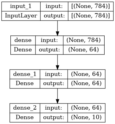
And, optionally, display the input and output shapes of each layer in the plotted graph:
keras.utils.plot_model(model, "my_first_model_with_shape_info.png", show_shapes=True)
This figure and the code are almost identical. In the code version, the connection arrows are replaced by the call operation.
A "graph of layers" is an intuitive mental image for a deep learning model, and the functional API is a way to create models that closely mirrors this.
Training, evaluation, and inference
Training, evaluation, and inference work exactly in the same way for models built using the functional API as for Sequential models.
The Model class offers a built-in training loop (the fit() method) and a built-in evaluation loop (the evaluate() method). Note that you can easily customize these loops to implement training routines beyond supervised learning (e.g. GANs).
Here, load the MNIST image data, reshape it into vectors, fit the model on the data (while monitoring performance on a validation split), then evaluate the model on the test data:
(x_train, y_train), (x_test, y_test) = keras.datasets.mnist.load_data()

x_train = x_train.reshape(60000, 784).astype("float32") / 255
x_test = x_test.reshape(10000, 784).astype("float32") / 255

model.compile(
    loss=keras.losses.SparseCategoricalCrossentropy(from_logits=True),
    optimizer=keras.optimizers.RMSprop(),
    metrics=[keras.metrics.SparseCategoricalAccuracy()],
)

history = model.fit(x_train, y_train, batch_size=64, epochs=2, validation_split=0.2)

test_scores = model.evaluate(x_test, y_test, verbose=2)
print("Test loss:", test_scores[0])
print("Test accuracy:", test_scores[1])
Epoch 1/2
750/750 [==============================] - 4s 3ms/step - loss: 0.3556 - sparse_categorical_accuracy: 0.8971 - val_loss: 0.1962 - val_sparse_categorical_accuracy: 0.9422
Epoch 2/2
750/750 [==============================] - 2s 2ms/step - loss: 0.1612 - sparse_categorical_accuracy: 0.9527 - val_loss: 0.1461 - val_sparse_categorical_accuracy: 0.9592
313/313 - 0s - loss: 0.1492 - sparse_categorical_accuracy: 0.9556 - 463ms/epoch - 1ms/step
Test loss: 0.14915992319583893
Test accuracy: 0.9556000232696533
For further reading, see the training and evaluation guide.
Save and serialize
Saving the model and serialization work the same way for models built using the functional API as they do for Sequential models. The standard way to save a functional model is to call model.save() to save the entire model as a single file. You can later recreate the same model from this file, even if the code that built the model is no longer available.
This saved file includes the:
- model architecture
- model weight values (that were learned during training)
- model training config, if any (as passed to
compile) - optimizer and its state, if any (to restart training where you left off)
model.save("path_to_my_model.keras")
del model
# Recreate the exact same model purely from the file:
model = keras.models.load_model("path_to_my_model.keras")
For details, read the model serialization & saving guide.
Use the same graph of layers to define multiple models
In the functional API, models are created by specifying their inputs and outputs in a graph of layers. That means that a single graph of layers can be used to generate multiple models.
In the example below, you use the same stack of layers to instantiate two models: an encoder model that turns image inputs into 16-dimensional vectors, and an end-to-end autoencoder model for training.
encoder_input = keras.Input(shape=(28, 28, 1), name="img")
x = layers.Conv2D(16, 3, activation="relu")(encoder_input)
x = layers.Conv2D(32, 3, activation="relu")(x)
x = layers.MaxPooling2D(3)(x)
x = layers.Conv2D(32, 3, activation="relu")(x)
x = layers.Conv2D(16, 3, activation="relu")(x)
encoder_output = layers.GlobalMaxPooling2D()(x)

encoder = keras.Model(encoder_input, encoder_output, name="encoder")
encoder.summary()

x = layers.Reshape((4, 4, 1))(encoder_output)
x = layers.Conv2DTranspose(16, 3, activation="relu")(x)
x = layers.Conv2DTranspose(32, 3, activation="relu")(x)
x = layers.UpSampling2D(3)(x)
x = layers.Conv2DTranspose(16, 3, activation="relu")(x)
decoder_output = layers.Conv2DTranspose(1, 3, activation="relu")(x)

autoencoder = keras.Model(encoder_input, decoder_output, name="autoencoder")
autoencoder.summary()
Model: "encoder"
_________________________________________________________________
 Layer (type)                Output Shape              Param #
=================================================================
 img (InputLayer)            [(None, 28, 28, 1)]       0

 conv2d (Conv2D)             (None, 26, 26, 16)        160

 conv2d_1 (Conv2D)           (None, 24, 24, 32)        4640

 max_pooling2d (MaxPooling2  (None, 8, 8, 32)          0
 D)

 conv2d_2 (Conv2D)           (None, 6, 6, 32)          9248

 conv2d_3 (Conv2D)           (None, 4, 4, 16)          4624

 global_max_pooling2d (Glob  (None, 16)                0
 alMaxPooling2D)

=================================================================
Total params: 18672 (72.94 KB)
Trainable params: 18672 (72.94 KB)
Non-trainable params: 0 (0.00 Byte)
_________________________________________________________________
Model: "autoencoder"
_________________________________________________________________
 Layer (type)                Output Shape              Param #
=================================================================
 img (InputLayer)            [(None, 28, 28, 1)]       0

 conv2d (Conv2D)             (None, 26, 26, 16)        160

 conv2d_1 (Conv2D)           (None, 24, 24, 32)        4640

 max_pooling2d (MaxPooling2  (None, 8, 8, 32)          0
 D)

 conv2d_2 (Conv2D)           (None, 6, 6, 32)          9248

 conv2d_3 (Conv2D)           (None, 4, 4, 16)          4624

 global_max_pooling2d (Glob  (None, 16)                0
 alMaxPooling2D)

 reshape (Reshape)           (None, 4, 4, 1)           0

 conv2d_transpose (Conv2DTr  (None, 6, 6, 16)          160
 anspose)

 conv2d_transpose_1 (Conv2D  (None, 8, 8, 32)          4640
 Transpose)

 up_sampling2d (UpSampling2  (None, 24, 24, 32)        0
 D)

 conv2d_transpose_2 (Conv2D  (None, 26, 26, 16)        4624
 Transpose)

 conv2d_transpose_3 (Conv2D  (None, 28, 28, 1)         145
 Transpose)

=================================================================
Total params: 28241 (110.32 KB)
Trainable params: 28241 (110.32 KB)
Non-trainable params: 0 (0.00 Byte)
_________________________________________________________________
Here, the decoding architecture is strictly symmetrical to the encoding architecture, so the output shape is the same as the input shape (28, 28, 1).
The reverse of a Conv2D layer is a Conv2DTranspose layer, and the reverse of a MaxPooling2D layer is an UpSampling2D layer.
All models are callable, just like layers
You can treat any model as if it were a layer by invoking it on an Input or on the output of another layer. By calling a model you aren't just reusing the architecture of the model, you're also reusing its weights.
To see this in action, here's a different take on the autoencoder example that creates an encoder model, a decoder model, and chains them in two calls to obtain the autoencoder model:
encoder_input = keras.Input(shape=(28, 28, 1), name="original_img")
x = layers.Conv2D(16, 3, activation="relu")(encoder_input)
x = layers.Conv2D(32, 3, activation="relu")(x)
x = layers.MaxPooling2D(3)(x)
x = layers.Conv2D(32, 3, activation="relu")(x)
x = layers.Conv2D(16, 3, activation="relu")(x)
encoder_output = layers.GlobalMaxPooling2D()(x)

encoder = keras.Model(encoder_input, encoder_output, name="encoder")
encoder.summary()

decoder_input = keras.Input(shape=(16,), name="encoded_img")
x = layers.Reshape((4, 4, 1))(decoder_input)
x = layers.Conv2DTranspose(16, 3, activation="relu")(x)
x = layers.Conv2DTranspose(32, 3, activation="relu")(x)
x = layers.UpSampling2D(3)(x)
x = layers.Conv2DTranspose(16, 3, activation="relu")(x)
decoder_output = layers.Conv2DTranspose(1, 3, activation="relu")(x)

decoder = keras.Model(decoder_input, decoder_output, name="decoder")
decoder.summary()

autoencoder_input = keras.Input(shape=(28, 28, 1), name="img")
encoded_img = encoder(autoencoder_input)
decoded_img = decoder(encoded_img)
autoencoder = keras.Model(autoencoder_input, decoded_img, name="autoencoder")
autoencoder.summary()
Model: "encoder"
_________________________________________________________________
 Layer (type)                Output Shape              Param #
=================================================================
 original_img (InputLayer)   [(None, 28, 28, 1)]       0

 conv2d_4 (Conv2D)           (None, 26, 26, 16)        160

 conv2d_5 (Conv2D)           (None, 24, 24, 32)        4640

 max_pooling2d_1 (MaxPoolin  (None, 8, 8, 32)          0
 g2D)

 conv2d_6 (Conv2D)           (None, 6, 6, 32)          9248

 conv2d_7 (Conv2D)           (None, 4, 4, 16)          4624

 global_max_pooling2d_1 (Gl  (None, 16)                0
 obalMaxPooling2D)

=================================================================
Total params: 18672 (72.94 KB)
Trainable params: 18672 (72.94 KB)
Non-trainable params: 0 (0.00 Byte)
_________________________________________________________________
Model: "decoder"
_________________________________________________________________
 Layer (type)                Output Shape              Param #
=================================================================
 encoded_img (InputLayer)    [(None, 16)]              0

 reshape_1 (Reshape)         (None, 4, 4, 1)           0

 conv2d_transpose_4 (Conv2D  (None, 6, 6, 16)          160
 Transpose)

 conv2d_transpose_5 (Conv2D  (None, 8, 8, 32)          4640
 Transpose)

 up_sampling2d_1 (UpSamplin  (None, 24, 24, 32)        0
 g2D)

 conv2d_transpose_6 (Conv2D  (None, 26, 26, 16)        4624
 Transpose)

 conv2d_transpose_7 (Conv2D  (None, 28, 28, 1)         145
 Transpose)

=================================================================
Total params: 9569 (37.38 KB)
Trainable params: 9569 (37.38 KB)
Non-trainable params: 0 (0.00 Byte)
_________________________________________________________________
Model: "autoencoder"
_________________________________________________________________
 Layer (type)                Output Shape              Param #
=================================================================
 img (InputLayer)            [(None, 28, 28, 1)]       0

 encoder (Functional)        (None, 16)                18672

 decoder (Functional)        (None, 28, 28, 1)         9569

=================================================================
Total params: 28241 (110.32 KB)
Trainable params: 28241 (110.32 KB)
Non-trainable params: 0 (0.00 Byte)
_________________________________________________________________
As you can see, the model can be nested: a model can contain sub-models (since a model is just like a layer). A common use case for model nesting is ensembling. For example, here's how to ensemble a set of models into a single model that averages their predictions:
def get_model():
    inputs = keras.Input(shape=(128,))
    outputs = layers.Dense(1)(inputs)
    return keras.Model(inputs, outputs)


model1 = get_model()
model2 = get_model()
model3 = get_model()

inputs = keras.Input(shape=(128,))
y1 = model1(inputs)
y2 = model2(inputs)
y3 = model3(inputs)
outputs = layers.average([y1, y2, y3])
ensemble_model = keras.Model(inputs=inputs, outputs=outputs)
Manipulate complex graph topologies
Models with multiple inputs and outputs
The functional API makes it easy to manipulate multiple inputs and outputs. This cannot be handled with the Sequential API.
For example, if you're building a system for ranking customer issue tickets by priority and routing them to the correct department, then the model will have three inputs:
- the title of the ticket (text input),
- the text body of the ticket (text input), and
- any tags added by the user (categorical input)
This model will have two outputs:
- the priority score between 0 and 1 (scalar sigmoid output), and
- the department that should handle the ticket (softmax output over the set of departments).
You can build this model in a few lines with the functional API:
num_tags = 12  # Number of unique issue tags
num_words = 10000  # Size of vocabulary obtained when preprocessing text data
num_departments = 4  # Number of departments for predictions

title_input = keras.Input(
    shape=(None,), name="title"
)  # Variable-length sequence of ints
body_input = keras.Input(shape=(None,), name="body")  # Variable-length sequence of ints
tags_input = keras.Input(
    shape=(num_tags,), name="tags"
)  # Binary vectors of size `num_tags`

# Embed each word in the title into a 64-dimensional vector
title_features = layers.Embedding(num_words, 64)(title_input)
# Embed each word in the text into a 64-dimensional vector
body_features = layers.Embedding(num_words, 64)(body_input)

# Reduce sequence of embedded words in the title into a single 128-dimensional vector
title_features = layers.LSTM(128)(title_features)
# Reduce sequence of embedded words in the body into a single 32-dimensional vector
body_features = layers.LSTM(32)(body_features)

# Merge all available features into a single large vector via concatenation
x = layers.concatenate([title_features, body_features, tags_input])

# Stick a logistic regression for priority prediction on top of the features
priority_pred = layers.Dense(1, name="priority")(x)
# Stick a department classifier on top of the features
department_pred = layers.Dense(num_departments, name="department")(x)

# Instantiate an end-to-end model predicting both priority and department
model = keras.Model(
    inputs=[title_input, body_input, tags_input],
    outputs=[priority_pred, department_pred],
)
Now plot the model:
keras.utils.plot_model(model, "multi_input_and_output_model.png", show_shapes=True)
When compiling this model, you can assign different losses to each output. You can even assign different weights to each loss -- to modulate their contribution to the total training loss.
model.compile(
    optimizer=keras.optimizers.RMSprop(1e-3),
    loss=[
        keras.losses.BinaryCrossentropy(from_logits=True),
        keras.losses.CategoricalCrossentropy(from_logits=True),
    ],
    loss_weights=[1.0, 0.2],
)
Since the output layers have different names, you could also specify the losses and loss weights with the corresponding layer names:
model.compile(
    optimizer=keras.optimizers.RMSprop(1e-3),
    loss={
        "priority": keras.losses.BinaryCrossentropy(from_logits=True),
        "department": keras.losses.CategoricalCrossentropy(from_logits=True),
    },
    loss_weights={"priority": 1.0, "department": 0.2},
)
Train the model by passing lists of NumPy arrays of inputs and targets:
# Dummy input data
title_data = np.random.randint(num_words, size=(1280, 10))
body_data = np.random.randint(num_words, size=(1280, 100))
tags_data = np.random.randint(2, size=(1280, num_tags)).astype("float32")

# Dummy target data
priority_targets = np.random.random(size=(1280, 1))
dept_targets = np.random.randint(2, size=(1280, num_departments))

model.fit(
    {"title": title_data, "body": body_data, "tags": tags_data},
    {"priority": priority_targets, "department": dept_targets},
    epochs=2,
    batch_size=32,
)
Epoch 1/2
40/40 [==============================] - 8s 112ms/step - loss: 1.2982 - priority_loss: 0.6991 - department_loss: 2.9958
Epoch 2/2
40/40 [==============================] - 3s 64ms/step - loss: 1.3110 - priority_loss: 0.6977 - department_loss: 3.0666
<keras.src.callbacks.History at 0x7f08d51fab80>
When calling fit with a Dataset object, it should yield either a tuple of lists like ([title_data, body_data, tags_data], [priority_targets, dept_targets]) or a tuple of dictionaries like ({'title': title_data, 'body': body_data, 'tags': tags_data}, {'priority': priority_targets, 'department': dept_targets}).
For more detailed explanation, refer to the training and evaluation guide.
A toy ResNet model
In addition to models with multiple inputs and outputs, the functional API makes it easy to manipulate non-linear connectivity topologies -- these are models with layers that are not connected sequentially, which the Sequential API cannot handle.
A common use case for this is residual connections. Let's build a toy ResNet model for CIFAR10 to demonstrate this:
inputs = keras.Input(shape=(32, 32, 3), name="img")
x = layers.Conv2D(32, 3, activation="relu")(inputs)
x = layers.Conv2D(64, 3, activation="relu")(x)
block_1_output = layers.MaxPooling2D(3)(x)

x = layers.Conv2D(64, 3, activation="relu", padding="same")(block_1_output)
x = layers.Conv2D(64, 3, activation="relu", padding="same")(x)
block_2_output = layers.add([x, block_1_output])

x = layers.Conv2D(64, 3, activation="relu", padding="same")(block_2_output)
x = layers.Conv2D(64, 3, activation="relu", padding="same")(x)
block_3_output = layers.add([x, block_2_output])

x = layers.Conv2D(64, 3, activation="relu")(block_3_output)
x = layers.GlobalAveragePooling2D()(x)
x = layers.Dense(256, activation="relu")(x)
x = layers.Dropout(0.5)(x)
outputs = layers.Dense(10)(x)

model = keras.Model(inputs, outputs, name="toy_resnet")
model.summary()
Model: "toy_resnet"
__________________________________________________________________________________________________
 Layer (type)                Output Shape                 Param #   Connected to
==================================================================================================
 img (InputLayer)            [(None, 32, 32, 3)]          0         []

 conv2d_8 (Conv2D)           (None, 30, 30, 32)           896       ['img[0][0]']

 conv2d_9 (Conv2D)           (None, 28, 28, 64)           18496     ['conv2d_8[0][0]']

 max_pooling2d_2 (MaxPoolin  (None, 9, 9, 64)             0         ['conv2d_9[0][0]']
 g2D)

 conv2d_10 (Conv2D)          (None, 9, 9, 64)             36928     ['max_pooling2d_2[0][0]']

 conv2d_11 (Conv2D)          (None, 9, 9, 64)             36928     ['conv2d_10[0][0]']

 add (Add)                   (None, 9, 9, 64)             0         ['conv2d_11[0][0]',
                                                                     'max_pooling2d_2[0][0]']

 conv2d_12 (Conv2D)          (None, 9, 9, 64)             36928     ['add[0][0]']

 conv2d_13 (Conv2D)          (None, 9, 9, 64)             36928     ['conv2d_12[0][0]']

 add_1 (Add)                 (None, 9, 9, 64)             0         ['conv2d_13[0][0]',
                                                                     'add[0][0]']

 conv2d_14 (Conv2D)          (None, 7, 7, 64)             36928     ['add_1[0][0]']

 global_average_pooling2d (  (None, 64)                   0         ['conv2d_14[0][0]']
 GlobalAveragePooling2D)

 dense_6 (Dense)             (None, 256)                  16640     ['global_average_pooling2d[0][
                                                                    0]']

 dropout (Dropout)           (None, 256)                  0         ['dense_6[0][0]']

 dense_7 (Dense)             (None, 10)                   2570      ['dropout[0][0]']

==================================================================================================
Total params: 223242 (872.04 KB)
Trainable params: 223242 (872.04 KB)
Non-trainable params: 0 (0.00 Byte)
__________________________________________________________________________________________________
Plot the model:
keras.utils.plot_model(model, "mini_resnet.png", show_shapes=True)
Now train the model:
(x_train, y_train), (x_test, y_test) = keras.datasets.cifar10.load_data()

x_train = x_train.astype("float32") / 255.0
x_test = x_test.astype("float32") / 255.0
y_train = keras.utils.to_categorical(y_train, 10)
y_test = keras.utils.to_categorical(y_test, 10)

model.compile(
    optimizer=keras.optimizers.RMSprop(1e-3),
    loss=keras.losses.CategoricalCrossentropy(from_logits=True),
    metrics=["acc"],
)
# We restrict the data to the first 1000 samples so as to limit execution time
# on Colab. Try to train on the entire dataset until convergence!
model.fit(x_train[:1000], y_train[:1000], batch_size=64, epochs=1, validation_split=0.2)
13/13 [==============================] - 4s 39ms/step - loss: 2.3086 - acc: 0.0988 - val_loss: 2.3020 - val_acc: 0.0850
<keras.src.callbacks.History at 0x7f078810c880>
Originally published on the