How to Define, Save, and Restore Models in TensorFlow

Content overview

• Setup
• TensorFlow Modules
• Building Modules
• Waiting to create variables
• Saving weights
• Saving functions
• Creating a SavedModel

To do machine learning in TensorFlow, you are likely to need to define, save, and restore a model.

A model is, abstractly:

• A function that computes something on tensors (a forward pass)
• Some variables that can be updated in response to training

In this guide, you will go below the surface of Keras to see how TensorFlow models are defined. This looks at how TensorFlow collects variables and models, as well as how they are saved and restored.

Setup

import tensorflow as tf
import keras
from datetime import datetime

%load_ext tensorboard

2023-10-18 01:21:05.536666: E tensorflow/compiler/xla/stream_executor/cuda/cuda_dnn.cc:9342] Unable to register cuDNN factory: Attempting to register factory for plugin cuDNN when one has already been registered
2023-10-18 01:21:05.536712: E tensorflow/compiler/xla/stream_executor/cuda/cuda_fft.cc:609] Unable to register cuFFT factory: Attempting to register factory for plugin cuFFT when one has already been registered
2023-10-18 01:21:05.536766: E tensorflow/compiler/xla/stream_executor/cuda/cuda_blas.cc:1518] Unable to register cuBLAS factory: Attempting to register factory for plugin cuBLAS when one has already been registered

TensorFlow Modules

Most models are made of layers. Layers are functions with a known mathematical structure that can be reused and have trainable variables. In TensorFlow, most high-level implementations of layers and models, such as Keras or Sonnet, are built on the same foundational class: tf.Module.

Building Modules

Here's an example of a very simple tf.Module that operates on a scalar tensor:

class SimpleModule(tf.Module):
  def __init__(self, name=None):
    super().__init__(name=name)
    self.a_variable = tf.Variable(5.0, name="train_me")
    self.non_trainable_variable = tf.Variable(5.0, trainable=False, name="do_not_train_me")
  def __call__(self, x):
    return self.a_variable * x + self.non_trainable_variable

simple_module = SimpleModule(name="simple")

simple_module(tf.constant(5.0))

2023-10-18 01:21:08.181350: W tensorflow/core/common_runtime/gpu/gpu_device.cc:2211] Cannot dlopen some GPU libraries. Please make sure the missing libraries mentioned above are installed properly if you would like to use GPU. Follow the guide at https://www.tensorflow.org/install/gpu for how to download and setup the required libraries for your platform.
Skipping registering GPU devices...
<tf.Tensor: shape=(), dtype=float32, numpy=30.0>

Modules and, by extension, layers are deep-learning terminology for "objects": they have internal state, and methods that use that state.

There is nothing special about __call__ except to act like a Python callable; you can invoke your models with whatever functions you wish.

You can set the trainability of variables on and off for any reason, including freezing layers and variables during fine-tuning.

By subclassing tf.Module, any tf.Variable or tf.Module instances assigned to this object's properties are automatically collected. This allows you to save and load variables, and also create collections of tf.Modules.

# All trainable variables
print("trainable variables:", simple_module.trainable_variables)
# Every variable
print("all variables:", simple_module.variables)

trainable variables: (<tf.Variable 'train_me:0' shape=() dtype=float32, numpy=5.0>,)
all variables: (<tf.Variable 'train_me:0' shape=() dtype=float32, numpy=5.0>, <tf.Variable 'do_not_train_me:0' shape=() dtype=float32, numpy=5.0>)

This is an example of a two-layer linear layer model made out of modules.

First a dense (linear) layer:

class Dense(tf.Module):
  def __init__(self, in_features, out_features, name=None):
    super().__init__(name=name)
    self.w = tf.Variable(
      tf.random.normal([in_features, out_features]), name='w')
    self.b = tf.Variable(tf.zeros([out_features]), name='b')
  def __call__(self, x):
    y = tf.matmul(x, self.w) + self.b
    return tf.nn.relu(y)

And then the complete model, which makes two layer instances and applies them:

class SequentialModule(tf.Module):
  def __init__(self, name=None):
    super().__init__(name=name)

    self.dense_1 = Dense(in_features=3, out_features=3)
    self.dense_2 = Dense(in_features=3, out_features=2)

  def __call__(self, x):
    x = self.dense_1(x)
    return self.dense_2(x)

# You have made a model!
my_model = SequentialModule(name="the_model")

# Call it, with random results
print("Model results:", my_model(tf.constant([[2.0, 2.0, 2.0]])))

Model results: tf.Tensor([[0.       3.415034]], shape=(1, 2), dtype=float32)

tf.Module instances will automatically collect, recursively, any tf.Variable or tf.Module instances assigned to it. This allows you to manage collections of tf.Modules with a single model instance, and save and load whole models.

print("Submodules:", my_model.submodules)

Submodules: (<__main__.Dense object at 0x7f7931aea250>, <__main__.Dense object at 0x7f77ed5b8a00>)

for var in my_model.variables:
  print(var, "\n")

<tf.Variable 'b:0' shape=(3,) dtype=float32, numpy=array([0., 0., 0.], dtype=float32)> 

<tf.Variable 'w:0' shape=(3, 3) dtype=float32, numpy=
array([[-2.8161757, -2.6065955,  1.9061812],
       [-0.9430401, -0.4624743, -0.4531979],
       [-1.3428234,  0.7062293,  0.7874674]], dtype=float32)> 

<tf.Variable 'b:0' shape=(2,) dtype=float32, numpy=array([0., 0.], dtype=float32)> 

<tf.Variable 'w:0' shape=(3, 2) dtype=float32, numpy=
array([[ 1.0474309 , -0.6920227 ],
       [ 1.2405277 ,  0.36411622],
       [-1.6990206 ,  0.762131  ]], dtype=float32)>

Waiting to create variables

You may have noticed here that you have to define both input and output sizes to the layer. This is so the w variable has a known shape and can be allocated.

By deferring variable creation to the first time the module is called with a specific input shape, you do not need specify the input size up front.

class FlexibleDenseModule(tf.Module):
  # Note: No need for `in_features`
  def __init__(self, out_features, name=None):
    super().__init__(name=name)
    self.is_built = False
    self.out_features = out_features

  def __call__(self, x):
    # Create variables on first call.
    if not self.is_built:
      self.w = tf.Variable(
        tf.random.normal([x.shape[-1], self.out_features]), name='w')
      self.b = tf.Variable(tf.zeros([self.out_features]), name='b')
      self.is_built = True

    y = tf.matmul(x, self.w) + self.b
    return tf.nn.relu(y)

# Used in a module
class MySequentialModule(tf.Module):
  def __init__(self, name=None):
    super().__init__(name=name)

    self.dense_1 = FlexibleDenseModule(out_features=3)
    self.dense_2 = FlexibleDenseModule(out_features=2)

  def __call__(self, x):
    x = self.dense_1(x)
    return self.dense_2(x)

my_model = MySequentialModule(name="the_model")
print("Model results:", my_model(tf.constant([[2.0, 2.0, 2.0]])))

Model results: tf.Tensor([[0. 0.]], shape=(1, 2), dtype=float32)

This flexibility is why TensorFlow layers often only need to specify the shape of their outputs, such as in tf.keras.layers.Dense, rather than both the input and output size.

Saving weights

You can save a tf.Module as both a checkpoint and a SavedModel.

Checkpoints are just the weights (that is, the values of the set of variables inside the module and its submodules):

chkp_path = "my_checkpoint"
checkpoint = tf.train.Checkpoint(model=my_model)
checkpoint.write(chkp_path)

'my_checkpoint'

Checkpoints consist of two kinds of files: the data itself and an index file for metadata. The index file keeps track of what is actually saved and the numbering of checkpoints, while the checkpoint data contains the variable values and their attribute lookup paths.

ls my_checkpoint*

my_checkpoint.data-00000-of-00001  my_checkpoint.index

You can look inside a checkpoint to be sure the whole collection of variables is saved, sorted by the Python object that contains them.

tf.train.list_variables(chkp_path)

[('_CHECKPOINTABLE_OBJECT_GRAPH', []),
 ('model/dense_1/b/.ATTRIBUTES/VARIABLE_VALUE', [3]),
 ('model/dense_1/w/.ATTRIBUTES/VARIABLE_VALUE', [3, 3]),
 ('model/dense_2/b/.ATTRIBUTES/VARIABLE_VALUE', [2]),
 ('model/dense_2/w/.ATTRIBUTES/VARIABLE_VALUE', [3, 2])]

During distributed (multi-machine) training they can be sharded, which is why they are numbered (e.g., '00000-of-00001'). In this case, though, there is only one shard.

When you load models back in, you overwrite the values in your Python object.

new_model = MySequentialModule()
new_checkpoint = tf.train.Checkpoint(model=new_model)
new_checkpoint.restore("my_checkpoint")

# Should be the same result as above
new_model(tf.constant([[2.0, 2.0, 2.0]]))

<tf.Tensor: shape=(1, 2), dtype=float32, numpy=array([[0., 0.]], dtype=float32)>

Saving functions

TensorFlow can run models without the original Python objects, as demonstrated by TensorFlow Serving and TensorFlow Lite, even when you download a trained model from TensorFlow Hub.

TensorFlow needs to know how to do the computations described in Python, but without the original code. To do this, you can make a graph, which is described in the Introduction to graphs and functions guide.

This graph contains operations, or ops, that implement the function.

You can define a graph in the model above by adding the @tf.function decorator to indicate that this code should run as a graph.

class MySequentialModule(tf.Module):
  def __init__(self, name=None):
    super().__init__(name=name)

    self.dense_1 = Dense(in_features=3, out_features=3)
    self.dense_2 = Dense(in_features=3, out_features=2)

  @tf.function
  def __call__(self, x):
    x = self.dense_1(x)
    return self.dense_2(x)

# You have made a model with a graph!
my_model = MySequentialModule(name="the_model")

The module you have made works exactly the same as before. Each unique signature passed into the function creates a separate graph. Check the Introduction to graphs and functions guide for details.

print(my_model([[2.0, 2.0, 2.0]]))
print(my_model([[[2.0, 2.0, 2.0], [2.0, 2.0, 2.0]]]))

tf.Tensor([[0.31593648 0.        ]], shape=(1, 2), dtype=float32)
tf.Tensor(
[[[0.31593648 0.        ]
  [0.31593648 0.        ]]], shape=(1, 2, 2), dtype=float32)

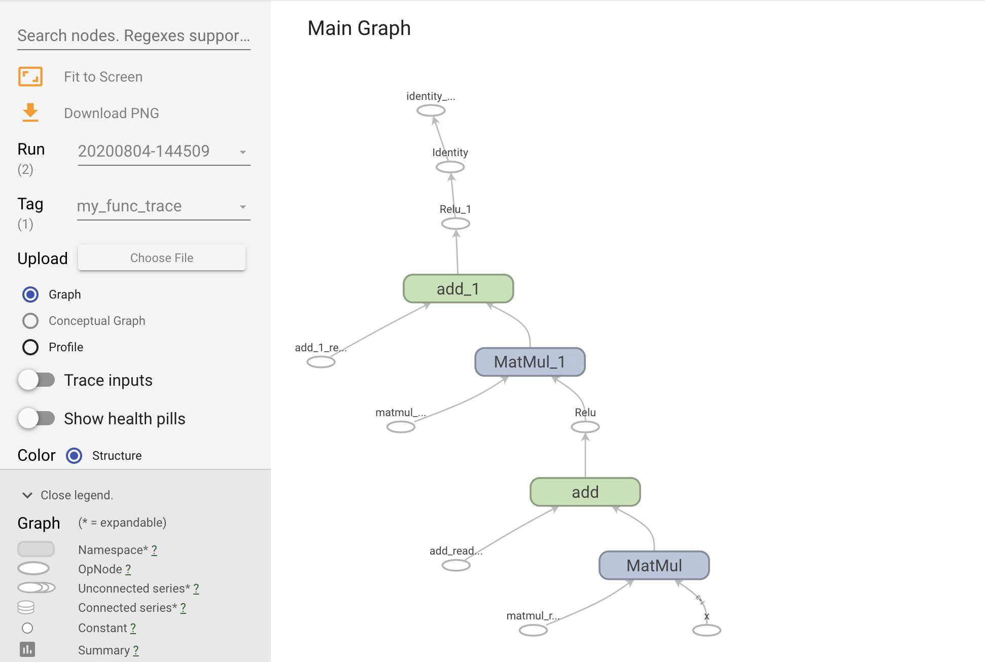
You can visualize the graph by tracing it within a TensorBoard summary.

# Set up logging.
stamp = datetime.now().strftime("%Y%m%d-%H%M%S")
logdir = "logs/func/%s" % stamp
writer = tf.summary.create_file_writer(logdir)

# Create a new model to get a fresh trace
# Otherwise the summary will not see the graph.
new_model = MySequentialModule()

# Bracket the function call with
# tf.summary.trace_on() and tf.summary.trace_export().
tf.summary.trace_on(graph=True)
tf.profiler.experimental.start(logdir)
# Call only one tf.function when tracing.
z = print(new_model(tf.constant([[2.0, 2.0, 2.0]])))
with writer.as_default():
  tf.summary.trace_export(
      name="my_func_trace",
      step=0,
      profiler_outdir=logdir)

tf.Tensor([[0. 0.]], shape=(1, 2), dtype=float32)

Launch TensorBoard to view the resulting trace:

#docs_infra: no_execute
%tensorboard --logdir logs/func

Creating a SavedModel

The recommended way of sharing completely trained models is to use SavedModel. SavedModel contains both a collection of functions and a collection of weights.

You can save the model you have just trained as follows:

tf.saved_model.save(my_model, "the_saved_model")

INFO:tensorflow:Assets written to: the_saved_model/assets

# Inspect the SavedModel in the directory
ls -l the_saved_model

total 32
drwxr-sr-x 2 kbuilder kokoro  4096 Oct 18 01:21 assets
-rw-rw-r-- 1 kbuilder kokoro    58 Oct 18 01:21 fingerprint.pb
-rw-rw-r-- 1 kbuilder kokoro 17704 Oct 18 01:21 saved_model.pb
drwxr-sr-x 2 kbuilder kokoro  4096 Oct 18 01:21 variables

# The variables/ directory contains a checkpoint of the variables
ls -l the_saved_model/variables

total 8
-rw-rw-r-- 1 kbuilder kokoro 490 Oct 18 01:21 variables.data-00000-of-00001
-rw-rw-r-- 1 kbuilder kokoro 356 Oct 18 01:21 variables.index

The saved_model.pb file is a protocol buffer describing the functional tf.Graph.

Models and layers can be loaded from this representation without actually making an instance of the class that created it. This is desired in situations where you do not have (or want) a Python interpreter, such as serving at scale or on an edge device, or in situations where the original Python code is not available or practical to use.

You can load the model as new object:

new_model = tf.saved_model.load("the_saved_model")

new_model, created from loading a saved model, is an internal TensorFlow user object without any of the class knowledge. It is not of type SequentialModule.

isinstance(new_model, SequentialModule)

False

This new model works on the already-defined input signatures. You can't add more signatures to a model restored like this.

print(my_model([[2.0, 2.0, 2.0]]))
print(my_model([[[2.0, 2.0, 2.0], [2.0, 2.0, 2.0]]]))

tf.Tensor([[0.31593648 0.        ]], shape=(1, 2), dtype=float32)
tf.Tensor(
[[[0.31593648 0.        ]
  [0.31593648 0.        ]]], shape=(1, 2, 2), dtype=float32)

Thus, using SavedModel, you are able to save TensorFlow weights and graphs using tf.Module, and then load them again.