How Toto Reimagines Multi-Head Attention for Multivariate Forecasting

Table of Links

1. Background
2. Problem statement
3. Model architecture
4. Training data
5. Results
6. Conclusions
7. Impact statement
8. Future directions
9. Contributions
10. Acknowledgements and References

Appendix

3 Model architecture

Toto is a decoder-only forecasting model. This model employs many of the latest techniques from the literature, and introduces a novel method for adapting multi-head attention to multivariate time series data (Fig. 1).

3.1 Transformer design

Transformer models for time series forecasting have variously used encoder-decoder [12, 13, 21], encoderonly [14, 15, 17], and decoder-only architectures [19, 23]. For Toto, we employ a decoder-only architecture. Decoder architectures have been shown to scale well [25, 26], and allow for arbitrary prediction horizons. The causal next-patch prediction task also simplifies the pre-training process.

We use techniques from some of the latest large language model (LLM) architectures, including prenormalization [27], RMSNorm [28], and SwiGLU feed-forward layers [29].

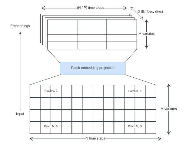
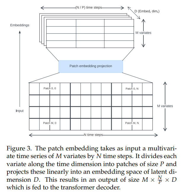
3.2 Input embedding

Time series transformers in the literature have used various approaches for creating input embeddings. We use non-overlapping patch projections (Fig. 3), first introduced for Vision Transformers [30, 31] and popularized in the time series context by PatchTST [14]. Toto was trained using a fixed patch size of 32.

3.3 Attention mechanism

Observability metrics are often high-cardinality, multivariate time series. Therefore, an ideal model will natively handle multivariate forecasting. It should be able to analyze relationships both in the time dimension (what we refer to as “time-wise” interactions) and in the channel dimension (what we refer to as “space-wise” interactions, following the convention in the Datadog platform of describing different groups or tag sets of a metric as the “space” dimension).

In order to model both space and time-wise interactions, we need to adapt the traditional multi-head attention architecture [11] from one to two dimensions. Several approaches have been proposed in the literature to do this, including:

• Assuming channel independence, and computing attention only in the time dimension [14]. This is efficient, but throws away all information about space-wise interactions.

• Computing attention only in the space dimension, and using a feed-forward network in the time dimension [17, 18].

• Concatenating variates along the time dimension and computing full cross-attention between every space/time location [15]. This can capture every possible space and time interaction, but it is computationally costly.

• Computing “factorized attention,” where each transformer block contains a separate space and time attention computation [16, 32, 33]. This allows both space and time mixing, and is more efficient than full cross-attention. However, it doubles the effective depth of the network.

In order to design our attention mechanism, we follow the intuition that for many time series, the time relationships are more important or predictive than the space relationships. As evidence, we observe that even models that completely ignore space-wise relationships (such as PatchTST [14] and TimesFM [19]) can still achieve competitive performance on multivariate datasets. However, other studies (e.g. Moirai [15]) have shown through ablations that there is some clear benefit to including space-wise relationships.

We therefore propose a novel variant of factorized attention, which we call “Proportional Factorized Space-Time Attention.” We use a mixture of alternating space-wise and time-wise attention blocks. As a configurable hyperparameter, we can change the ratio of time-wise to space-wise blocks, thus allowing us to devote more or less compute budget to each type of attention. For our base model, we selected a configuration with one space-wise attention block for every two time-wise blocks.

In the time-wise attention blocks, we use causal masking and rotary positional embeddings [34] with XPOS [35] in order to autoregressively model timedependent features. In the space-wise blocks, by contrast, we use full bidirectional attention in order to preserve permutation invariance of the covariates, with a block-diagonal ID mask to ensure that only related variates attend to each other. This masking allows us to pack multiple independent multivariate time series into the same batch, in order to improve training efficiency and reduce the amount of padding.

3.4 Probabilistic prediction head

In order to be useful for forecasting applications, a model should produce probabilistic predictions. A common practice in time series models is to use an output layer where the model regresses the parameters of a probability distribution. This allows for prediction intervals to be computed using Monte Carlo sampling [7].

Common choices for an output layer are Normal [7] and Student-T [23, 36], which can improve robustness to outliers. Moirai [15] allows for more flexible residual distributions by proposing a novel mixture model incorporating a weighted combination of Gaussian, Student-T, Log-Normal, and Negative-Binomial outputs.

However, real-world time series can often have complex distributions that are challenging to fit, with outliers, heavy tails, extreme skew, and multimodality. In order to accommodate these scenarios, we introduce an even more flexible output likelihood. To do this we employ a method based on Gaussian mixture models (GMMs), which can approximate any density function ([37]). To avoid training instability in the presence of outliers, we use a Student-T mixture model (SMM), a robust generalization of GMMs [38] that has previously shown promise for modeling heavy-tailed financial time series [39, 40]. The model predicts k Student-T distributions (where k is a hyperparameter) for each time step, as well as a learned weighting.

When we perform inference, we draw samples from the mixture distribution at each timestamp, then feed each sample back into the decoder for the next prediction. This allows us to produce prediction intervals at any quantile, limited only by the number of samples; for more precise tails, we can choose to spend more computation on sampling (Fig. 2).

3.5 Input/output scaling

As in other time series models, we perform instance normalization on input data before passing it through the patch embedding, in order to make the model generalize better to inputs of different scales [41]. We scale the inputs to have zero mean and unit standard deviation. The output predictions are then rescaled back to the original units.

3.6 Training objective

As a decoder-only model, Toto is pre-trained on the next-patch prediction task. We minimize the negative log-likelihood of the next predicted patch with respect to the distribution output of the model. We train the model using the AdamW optimizer [42].

3.7 Hyperparameters

The hyperparameters used for Toto are detailed in Table A.1, with 103 million total parameters.