Learn how tensorflow or pytorch implement optimization algorithms by using numpy and create beautiful animations using matplotlib

In this post, we will discuss how to implement different variants of gradient descent optimization technique and also visualize the working of the update rule for these variants using matplotlib. This is a follow-up to my previous post on optimization algorithms.

Citation Note: The content and the structure of this article is based on the deep learning lectures from One-Fourth Labs — PadhAI.

Gradient Descent is one of the most commonly used optimization techniques to optimize neural networks. Gradient descent algorithm updates the parameters by moving in the direction opposite to the gradient of the objective function with respect to the network parameters.

https://hackernoon.com/demystifying-different-variants-of-gradient-descent-optimization-algorithm-19ae9ba2e9bc

Implementation In Python Using Numpy

Photo by Christopher Gower on Unsplash

In the coding part, we will be covering the following topics.

Sigmoid Neuron Class
Overall setup — What is the data, model, task
Plotting functions — 3D & contour plots
Individual algorithms and how they perform

Individual Algorithms include,

Batch Gradient DescentMomentum GDNesterov Accelerated GDMini Batch and Stochastic GDAdaGrad GDRMSProp GDAdam GD

If you want to skip the theory part and get into the code right away,

https://github.com/Niranjankumar-c/GradientDescent_Implementation?source=post_page-----809e7ab3bab4----------------------

Before we start implementing gradient descent, first we need to import the required libraries. We are importing

Axes3D

from

mpl_toolkits.mplot3d

provides some basic 3D plotting (scatter, surf, line, mesh) tools. Not the fastest or most feature complete 3D library out there, but it ships with Matplotlib. we are also importing

colors

and

colormap(cm)

from Matplotlib. We would like to have animated plots to demonstrate how each optimization algorithm works, so we are importing

animation

and

rc

to make graphs look good. To display/render

HTML

content in-line in jupyter notebook import HTML. Finally, import

numpy

for computation purposes which does the most of our heavy lifting.

from mpl_toolkits.mplot3d import Axes3D
import matplotlib.pyplot as plt

from matplotlib import cm
import matplotlib.colors

from matplotlib import animation, rc
from IPython.display import HTML

import numpy as np

View codes on Github

Sigmoid Neuron Implementation

To implement the gradient descent optimization technique, we will take a simple case of the sigmoid neuron(logistic function) and see how different variants of gradient descent learns the parameters ‘w’ and ‘b’.

Sigmoid Neuron Recap

A sigmoid neuron is similar to the perceptron neuron, for every input xi it has weight wi associated with the input. The weights indicate the importance of the input in the decision-making process. The output from the sigmoid is not 0 or 1 like the perceptron model instead it is a real value between 0–1 which can be interpreted as a probability. The most commonly used sigmoid function is the logistic function, which has a characteristic of an “S” shaped curve.

Sigmoid Neuron Representation (logistic function)

Learning Algorithm

The objective of the learning algorithm is to determine the best possible values for the parameters (w and b), such that the overall loss (squared error loss) of the model is minimized as much as possible.

We initialize w and b randomly. We then iterate over all the observations in the data, for each observation find the corresponding predicted the outcome using the sigmoid function and compute the mean squared error loss. Based on the loss value, we will update the weights such that the overall loss of the model at the new parameters will be less than the current loss of the model.

To understand the math behind the gradient descent optimization technique, kindly go through my previous article on the sigmoid neuron learning algorithm — linked at the end of this article.

Sigmoid Neuron Class

Before we start analyzing different variants of gradient descent algorithm, We will build our model inside a class called SN.

class SN:
  #constructor
  def __init__(self, w_init, b_init, algo):
    self.w = w_init
    self.b = b_init
    self.w_h = []
    self.b_h = []
    self.e_h = []
    self.algo = algo
  #logistic function  
  def sigmoid(self, x, w=None, b=None):
    if w is None:
      w = self.w
    if b is None:
      b = self.b
    return 1. / (1. + np.exp(-(w*x + b)))
  #loss function
  def error(self, X, Y, w=None, b=None):
    if w is None:
      w = self.w
    if b is None:
      b = self.b
    err = 0
    for x, y in zip(X, Y):
      err += 0.5 * (self.sigmoid(x, w, b) - y) ** 2
    return err
  
  def grad_w(self, x, y, w=None, b=None):
    if w is None:
      w = self.w
    if b is None:
      b = self.b
    y_pred = self.sigmoid(x, w, b)
    return (y_pred - y) * y_pred * (1 - y_pred) * x
  
  def grad_b(self, x, y, w=None, b=None):
    if w is None:
      w = self.w
    if b is None:
      b = self.b
    y_pred = self.sigmoid(x, w, b)
    return (y_pred - y) * y_pred * (1 - y_pred)
  
  def fit(self, X, Y, 
          epochs=100, eta=0.01, gamma=0.9, mini_batch_size=100, eps=1e-8,  
          beta=0.9, beta1=0.9, beta2=0.9
         ):
    self.w_h = []
    self.b_h = []
    self.e_h = []
    self.X = X
    self.Y = Y
    
    if self.algo == 'GD':
      for i in range(epochs):
        dw, db = 0, 0
        for x, y in zip(X, Y):
          dw += self.grad_w(x, y)
          db += self.grad_b(x, y)
        self.w -= eta * dw / X.shape[0]
        self.b -= eta * db / X.shape[0]
        self.append_log()
        
    elif self.algo == 'MiniBatch':
      for i in range(epochs):
        dw, db = 0, 0
        points_seen = 0
        for x, y in zip(X, Y):
          dw += self.grad_w(x, y)
          db += self.grad_b(x, y)
          points_seen += 1
          if points_seen % mini_batch_size == 0:
            self.w -= eta * dw / mini_batch_size
            self.b -= eta * db / mini_batch_size
            self.append_log()
            dw, db = 0, 0
        
    elif self.algo == 'Momentum':
      v_w, v_b = 0, 0
      for i in range(epochs):
        dw, db = 0, 0
        for x, y in zip(X, Y):
          dw += self.grad_w(x, y)
          db += self.grad_b(x, y)
        v_w = gamma * v_w + eta * dw 
        v_b = gamma * v_b + eta * db
        self.w = self.w - v_w
        self.b = self.b - v_b
        self.append_log()
        
    elif self.algo == 'NAG':
      v_w, v_b = 0, 0
      for i in range(epochs):
        dw, db = 0, 0
        v_w = gamma * v_w
        v_b = gamma * v_b
        for x, y in zip(X, Y):
          dw += self.grad_w(x, y, self.w - v_w, self.b - v_b)
          db += self.grad_b(x, y, self.w - v_w, self.b - v_b)
        v_w = v_w + eta * dw
        v_b = v_b + eta * db
        self.w = self.w - v_w
        self.b = self.b - v_b
        self.append_log()
   #logging      
  def append_log(self):
    self.w_h.append(self.w)
    self.b_h.append(self.b)
    self.e_h.append(self.error(self.X, self.Y))

View on Github

#constructor  
def __init__(self, w_init, b_init, algo):    
    self.w = w_init    
    self.b = b_init    
    self.w_h = []    
    self.b_h = []    
    self.e_h = []    
    self.algo = algo

The

__init__

function (constructor function) helps to initialize the parameters of sigmoid neuron w weights and b biases. The function takes three arguments,

```
w_init,b_init
```
— These parameters take the initial values for the parameters ‘w’ and ‘b’ instead of setting parameters randomly, we are setting it to specific values. This allows us to understand how an algorithm performs by visualizing for different initial points. Some algorithms get stuck in local minima at some parameters.
```
algo
```
— It tells which variant of gradient descent algorithm to use for finding the optimal parameters.

In this function, we are initializing the parameters and we have defined three new array variables suffixed with ‘_h’ denoting that they are history variables, to keep track of how weights (w_h), biases (b_h) and error (e_h) values are changing as the sigmoid neuron learns the parameters.

def sigmoid(self, x, w=None, b=None):
    if w is None:
      w = self.w
    if b is None:
      b = self.b
    return 1. / (1. + np.exp(-(w*x + b)))

We have thesigmoid function that takes input x — mandatory argument and computes the logistic function for the input along with the parameters. The function also takes two other optional arguments.

```
w & b
```
—By taking ‘w’ and ‘b’ as the parameters it helps us to calculate the value of the sigmoid function at specifically specified values of parameters. If these arguments are not passed, it will take the values of learned parameters to compute the logistic function.

def error(self, X, Y, w=None, b=None):
    if w is None:
      w = self.w
    if b is None:
      b = self.b
    err = 0
    for x, y in zip(X, Y):
      err += 0.5 * (self.sigmoid(x, w, b) - y) ** 2
    return err

Next, we have

error

function that takes input X and Y as mandatory arguments and optional parameter arguments like in the

sigmoid

function. In this function, we are iterating through each data point and computing the cumulative mean squared error between the actual feature value and predicted feature value using the

sigmoid

function. Like we have seen in the sigmoid function, it has support for calculating the error at specified parameter values.

def grad_w(self, x, y, w=None, b=None):
   .....
def grad_b(self, x, y, w=None, b=None):
   .....

Next, we will define two functions

grad_w

and

grad_b

takes input ‘x’ and ‘y’ as mandatory arguments, which helps to compute the gradient of the sigmoid with respect to inputs for the parameters ‘w’ and ‘b’ respectively. Again we have two optional arguments that allow us to compute the gradient at specified parameter values.

def fit(self, X, Y, epochs=100, eta=0.01, gamma=0.9, mini_batch_size=100, eps=1e-8,beta=0.9, beta1=0.9, beta2=0.9):
    self.w_h = []
    .......

Next, we define the ‘fit’ method that takes inputs ‘X’, ‘Y’ and a bunch of other parameters. I will explain these parameters whenever it is being used for a particular variant of gradient descent algorithm. The function starts by initializing the history variables and setting the local input variables to store the input parameter data.

Then we have a bunch of different ‘if-else’ statements for each algorithm it supports. Depending on the algorithm we use to choose, we will implement the gradient descent in the fit function. I will explain each of these implementations in detail in the later part of the article.

def append_log(self):
    self.w_h.append(self.w)
    self.b_h.append(self.b)
    self.e_h.append(self.error(self.X, self.Y))

Finally, we have

theappend_log

function to store the value of parameters and loss function value for each epoch in each variant of gradient descent.

Setting Up for Plotting

In this section, we will define some configuration parameters for simulating the gradient descent update rule using a simple 2D toy data set. We also define some functions to create and animate the 3D & 2D plots to visualize the working of update rule. This kind of setup helps us to run different experiments with different starting points, different hyperparameter settings and plot/animate update rule for different variants of the gradient descent.

#Data
X = np.asarray([3.5, 0.35, 3.2, -2.0, 1.5, -0.5])
Y = np.asarray([0.5, 0.50, 0.5,  0.5, 0.1,  0.3])
#Algo and parameter values
algo = 'GD'
w_init = 2.1
b_init = 4.0
#parameter min and max values- to plot update rule
w_min = -7
w_max = 5
b_min = -7
b_max = 5
#learning algorithum options
epochs = 200
mini_batch_size = 6
gamma = 0.9
eta = 5
#animation number of frames
animation_frames = 20
#plotting options
plot_2d = True
plot_3d = False

First, we take a simple 2D toy data set that has two inputs and two outputs. In line 5, we define a string variable algo that takes which type of algorithm we want to execute. We initialize the parameters ‘w’ and ‘b’ in Line 6 — 7 to indicate where the algorithm starts.

From line 9 — 12 we are setting the limits for the parameters, the range where sigmoid neuron searches for the best parameters within the specified range. These numbers are specifically chosen well to illustrate the working gradient descent update rule. Next, we are setting values of hyperparameters some variables will be specific to some algorithms, I will discuss them when we are discussing the implementation of algorithms. Finally, from line 19–22, we declared the variables required to animate or plot the update rule.

sn = SN(w_init, b_init, algo)
sn.fit(X, Y, epochs=epochs, eta=eta, gamma=gamma, mini_batch_size=mini_batch_size)
plt.plot(sn.e_h, 'r')
plt.plot(sn.w_h, 'b')
plt.plot(sn.b_h, 'g')
plt.legend(('error', 'weight', 'bias'))
plt.title("Variation of Parameters and loss function")
plt.xlabel("Epoch")
plt.show()

Once we set up our configuration parameters, we will initialize our SN class and then call the fit method using the configuration parameters. We also plot our three history variables to visualize how the parameters and loss function value varies across epochs.

3D & 2D Plotting Setup

if plot_3d: 
  W = np.linspace(w_min, w_max, 256)
  b = np.linspace(b_min, b_max, 256)
  WW, BB = np.meshgrid(W, b)
  Z = sn.error(X, Y, WW, BB)

  fig = plt.figure(dpi=100)
  ax = fig.gca(projection='3d')
  surf = ax.plot_surface(WW, BB, Z, rstride=3, cstride=3, alpha=0.5, cmap=cm.coolwarm, linewidth=0, antialiased=False)
  cset = ax.contourf(WW, BB, Z, 25, zdir='z', offset=-1, alpha=0.6, cmap=cm.coolwarm)
  ax.set_xlabel('w')
  ax.set_xlim(w_min - 1, w_max + 1)
  ax.set_ylabel('b')
  ax.set_ylim(b_min - 1, b_max + 1)
  ax.set_zlabel('error')
  ax.set_zlim(-1, np.max(Z))
  ax.view_init (elev=25, azim=-75) # azim = -20
  ax.dist=12  
  title = ax.set_title('Epoch 0')

To create a 3D plot first, we create a mesh grid by creating 256 equally spaced values between the minimum and maximum values of ‘w’ and ‘b’ as shown in line 2–5. Using the mesh grid will calculate the error (line 5) for these values by calling the

error

function in our sigmoid class

SN

. In line 8, we are creating an axis handle to create a 3D plot.

To create a 3D plot, we are creating a surface plot of the error with respect to weight and bias using

ax.plot_surface

function by specifying how often we want to sample the points along with the data by setting

rstride

and

cstride

. Next, we are plotting the contour of the error with respect to weight and bias on top of the surface using ax.contourf function by specifying error values as ‘Z’ direction (Line 9 — 10). In line 11–16, we are setting the labels for each axis and axis limits for all three dimensions. Because we are plotting the 3D plot, we need to define the viewpoint. In line 17–18 we are setting a viewpoint for our plot at an elevation of 25 degrees in the ‘z’ axis and at a distance of 12 units.

def plot_animate_3d(i):
  i = int(i*(epochs/animation_frames))
  line1.set_data(sn.w_h[:i+1], sn.b_h[:i+1])
  line1.set_3d_properties(sn.e_h[:i+1])
  line2.set_data(sn.w_h[:i+1], sn.b_h[:i+1])
  line2.set_3d_properties(np.zeros(i+1) - 1)
  title.set_text('Epoch: {: d}, Error: {:.4f}'.format(i, sn.e_h[i]))
  return line1, line2, title

if plot_3d: 
  #animation plots of gradient descent
  i = 0
  line1, = ax.plot(sn.w_h[:i+1], sn.b_h[:i+1], sn.e_h[:i+1], color='black',marker='.')
  line2, = ax.plot(sn.w_h[:i+1], sn.b_h[:i+1], np.zeros(i+1) - 1, color='red', marker='.')
  anim = animation.FuncAnimation(fig, func=plot_animate_3d, frames=animation_frames)
  rc('animation', html='jshtml')
  anim

On top of our static 3D plot, we want to visualize what the algorithm is doing dynamically which is captured by our history variables for parameters and error function at every epoch of our algorithm. To create an animation of our gradient descent algorithm, we will use

animation.FuncAnimation

function by passing our custom function

plot_animate_3d

as one of the parameters and also specify the number of frames needed to create an animation. The function

plot_animate_3d

updates the values of parameters and error value for the respective values of ‘w’ and ‘b’. In the same function at the line — 7, we are setting the text to show the error value at that particular epoch. Finally, to display the animation in-line we call the

rc

function to render the HTML content inside the jupyter notebook.

Similar to the 3D plot, we can create a function to plot 2D contour plots.

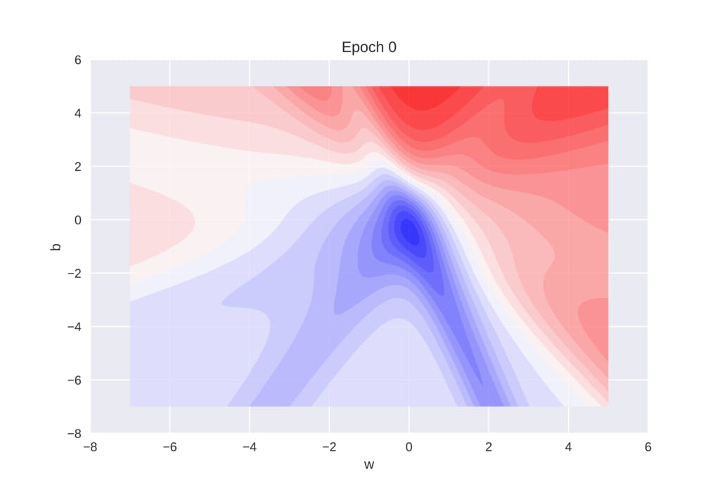
if plot_2d: 
  W = np.linspace(w_min, w_max, 256)
  b = np.linspace(b_min, b_max, 256)
  WW, BB = np.meshgrid(W, b)
  Z = sn.error(X, Y, WW, BB)

  fig = plt.figure(dpi=100)
  ax = plt.subplot(111)
  ax.set_xlabel('w')
  ax.set_xlim(w_min - 1, w_max + 1)
  ax.set_ylabel('b')
  ax.set_ylim(b_min - 1, b_max + 1)
  title = ax.set_title('Epoch 0')
  cset = plt.contourf(WW, BB, Z, 25, alpha=0.8, cmap=cm.bwr)
  plt.savefig("temp.jpg",dpi = 2000)
  plt.show()

def plot_animate_2d(i):
  i = int(i*(epochs/animation_frames))
  line.set_data(sn.w_h[:i+1], sn.b_h[:i+1])
  title.set_text('Epoch: {: d}, Error: {:.4f}'.format(i, sn.e_h[i]))
  return line, title

if plot_2d: 
  i = 0
  line, = ax.plot(sn.w_h[:i+1], sn.b_h[:i+1], color='black',marker='.')
  anim = animation.FuncAnimation(fig, func=plot_animate_2d, frames=animation_frames)
  rc('animation', html='jshtml')
  anim

Algorithm Implementation

In this section, we will implement different variants of gradient descent algorithm and generate 3D & 2D animation plots.

Vanilla Gradient Descent

Gradient descent algorithm updates the parameters by moving in the direction opposite to the gradient of the objective function with respect to the network parameters.

Parameter update rule will be given by,

Gradient Descent Update Rule

for i in range(epochs):
        dw, db = 0, 0
        for x, y in zip(X, Y):
          dw += self.grad_w(x, y)
          db += self.grad_b(x, y)
        self.w -= eta * dw / X.shape[0]
        self.b -= eta * db / X.shape[0]
        self.append_log()

In the batch gradient descent, we iterate over all the training data points and compute the cumulative sum of gradients for parameters ‘w’ and ‘b’. Then update the values of parameters based on the cumulative gradient value and the learning rate.

To execute the gradient descent algorithm change the configuration settings as shown below.

X = np.asarray([0.5, 2.5])
Y = np.asarray([0.2, 0.9])

algo = 'GD'
w_init = -2
b_init = -2
w_min = -7
w_max = 5
b_min = -7
b_max = 5

epochs = 1000
eta = 1

animation_frames = 20

plot_2d = True
plot_3d = True

In the configuration settings, we are setting the variable

algo

to ‘GD’ to indicate we want to execute the vanilla gradient descent algorithm in our sigmoid neuron to find the best parameter values. After we set up our configuration parameters, we will go ahead and execute the SN class ‘fit’ method to train sigmoid neuron on toy data.

Gradient Descent History

The above plot shows how the history values of error, weight, and bias vary across different epochs while the algorithm is learning the best parameters. The important point to note from the graph is that during the initial epochs error value is hovering close to 0.5 but after 200 epochs the error values reaches almost zero.

If you want to plot 3D or 2D animation, you can set the boolean variables

plot_2d

and

plot_3d

. I will show how the 3D error surface would look like for corresponding values of ‘w’ and ‘b’. The objective of the learning algorithm is to move towards the deep blue color region where the error/loss is minimum.

To visualize what algorithm is doing dynamically, we can generate an animation by using the function

plot_animate_3d

. As you play the animation, you can see the epoch number and the corresponding error value at that epoch.

If you want to slow down the animation, you can do that by clicking on the minus symbol in the video controls as shown in the above animation. Similarly, you can generate the animation for 2D contour plot to see how the algorithm is moving towards the global minima.

Momentum-based Gradient Descent

In Momentum GD, we are moving with an exponential decaying cumulative average of previous gradients and current gradient.

The code for the Momentum GD is given below,

v_w, v_b = 0, 0
for i in range(epochs):
  dw, db = 0, 0
 for x, y in zip(X, Y):
   dw += self.grad_w(x, y)
   db += self.grad_b(x, y)
 v_w = gamma * v_w + eta * dw 
 v_b = gamma * v_b + eta * db
 self.w = self.w - v_w
 self.b = self.b - v_b
 self.append_log()

In Momentum based GD, we have included the history variable to keep track of the values of previous gradients. The variable gamma denotes the how much of momentum we need to impart to the algorithm. The variables

v_w

and

v_b

will be used to compute the movement of the gradient based on the history as well as the current gradient. At the end of each epoch, we are calling the

append_log

function to store the history of parameters and loss function values.

To execute the Momentum GD for our sigmoid neuron, you need to make few modifications to the configuration settings as shown below,

X = np.asarray([0.5, 2.5])
Y = np.asarray([0.2, 0.9])
algo = 'Momentum'
w_init = -2
b_init = -2
w_min = -7
w_max = 5
b_min = -7
b_max = 5
epochs = 1000
mini_batch_size = 6
gamma = 0.9
eta = 1
animation_frames = 20
plot_2d = True
plot_3d = True

The variable

algo

is set to ‘Momentum’ to indicate that we want to use the Momentum GD for finding the best parameters for our sigmoid neuron and another important change is the

gamma

variable, which is used to control how much momentum we need to impart into the learning algorithm. Gamma value varies between 0–1. After we set up our configuration parameters, we will go ahead and execute the SN class ‘fit’ method to train sigmoid neuron on toy data.

Variation for Momentum GD

From the plot, we can see that there were a lot of oscillations in the values of weight and bias terms because of the accumulated history Momentum GD oscillates in and out of minima.

Nesterov Accelerated Gradient Descent

In Nesterov Accelerated Gradient Descent we are looking forward to seeing whether we are close to the minima or not before we take another step based on the current gradient value so that we can avoid the problem of overshooting.

The code for the Momentum GD is given below,

v_w, v_b = 0, 0
for i in range(epochs):
  dw, db = 0, 0
 v_w = gamma * v_w
 v_b = gamma * v_b
 for x, y in zip(X, Y):
   dw += self.grad_w(x, y, self.w - v_w, self.b - v_b)
   db += self.grad_b(x, y, self.w - v_w, self.b - v_b)
 v_w = v_w + eta * dw
 v_b = v_b + eta * db
 self.w = self.w - v_w
 self.b = self.b - v_b
 self.append_log()

The main change in the code for NAG GD is that the computation of

v_w

and

v_b

. In Momentum GD, we are computing these variables in one step but in NAG we are doing it in two steps.

v_w = gamma * v_w
v_b = gamma * v_b
for x, y in zip(X, Y):
   dw += self.grad_w(x, y, self.w - v_w, self.b - v_b)
   db += self.grad_b(x, y, self.w - v_w, self.b - v_b)
 v_w = v_w + eta * dw
 v_b = v_b + eta * db

In the first part, before we iterate through the data, we will multiply the gamma with our history variables and then the gradient is computed by using the subtracted history value from

self.w

and

self.b

. To execute the NAG GD, we need just need to set the

algo

variable to ‘NAG’. You can generate the 3D or 2D animations to see how the NAG GD is different from Momentum GD in reaching the global minima.

Mini-Batch and Stochastic Gradient Descent

Instead of looking at all data points at one go, we will divide the entire data into a number of subsets. For each subset of data, compute the derivates for each of the point present in the subset and make an update to the parameters. Instead of calculating the derivative for entire data with respect to the loss function, we have approximated it to fewer points or smaller batch size. This method of computing gradients in batches is called the Mini-Batch Gradient Descent

The code for the Mini-Batch GD is given below,

for i in range(epochs):
dw, db = 0, 0
points_seen = 0
for x, y in zip(X, Y):
  dw += self.grad_w(x, y)
  db += self.grad_b(x, y)
  points_seen += 1
  if points_seen % mini_batch_size == 0:
     self.w -= eta * dw / mini_batch_size
     self.b -= eta * db / mini_batch_size
     self.append_log()
     dw, db = 0, 0

In Mini Batch, we are looping through the entire data and keeping track of the number of points we have seen by using a variable points_seen. If the number of points seen is a multiple of mini-batch size then we are updating the parameters of the sigmoid neuron. In the special case when mini-batch size is equal to one, then it would become Stochastic Gradient Descent. To execute the Mini-Batch GD, we need just need to set the algo variable to ‘MiniBatch’. You can generate the 3D or 2D animations to see how the Mini-Batch GD is different from Momentum GD in reaching the global minima.

AdaGrad Gradient Descent

The main motivation behind the AdaGrad was the idea of Adaptive Learning rate for different features in the dataset, i.e. instead of using the same learning rate across all the features in the dataset, we might need different learning rate for different features.

The code for Adagrad is given below,

v_w, v_b = 0, 0
for i in range(epochs):
 dw, db = 0, 0
 for x, y in zip(X, Y):
   dw += self.grad_w(x, y)
   db += self.grad_b(x, y)
 v_w += dw**2
 v_b += db**2
 self.w -= (eta / np.sqrt(v_w) + eps) * dw
 self.b -= (eta / np.sqrt(v_b) + eps) * db
 self.append_log()

In Adagrad, we are maintaining the running squared sum of gradients and then we update the parameters by dividing the learning rate with the square root of the historical values. Instead of having a static learning rate here we have dynamic learning for dense and sparse features. The mechanism to generate plots/animation remains the same as above. The idea here is to play with different toy datasets and different hyperparameter configurations.

RMSProp Gradient Descent

In RMSProp history of gradients is calculated using an exponentially decaying average unlike the sum of gradients in AdaGrad, which helps to prevent the rapid growth of the denominator for dense features.

The code for RMSProp is given below,

v_w, v_b = 0, 0
for i in range(epochs):
 dw, db = 0, 0
 for x, y in zip(X, Y):
   dw += self.grad_w(x, y)
   db += self.grad_b(x, y)
 v_w = beta * v_w + (1 - beta) * dw**2
 v_b = beta * v_b + (1 - beta) * db**2
 self.w -= (eta / np.sqrt(v_w) + eps) * dw
 self.b -= (eta / np.sqrt(v_b) + eps) * db
 self.append_log()

The only change we need to do in AdaGrad code is how we update the variables

v_w

and

v_b

. In AdaGrad

v_w

and v_b is always increasing by squares of the gradient per parameter wise since the first epoch but in RMSProp

v_w

and

v_b

is exponentially decaying weighted sum of gradients by using a hyperparameter called ‘gamma’. To execute the RMSProp GD, we need just need to set the algo variable to ‘RMSProp’. You can generate the 3D or 2D animations to see how the RMSProp GD is different from AdaGrad GD in reaching the global minima.

Adam Gradient Descent

Adam maintains two histories, ‘mₜ’ similar to the history used in Momentum GD and ‘vₜ’ similar to the history used in RMSProp.

In practice, Adam does something known as bias correction. It uses the following equations for ‘mₜ’ and ‘vₜ’,

Bias Correction

Bias correction ensures that at the beginning of the training updates don’t behave in a weird manner. The key point in Adam is that it combines the advantages of Momentum GD (moving faster in gentle regions) and RMSProp GD (adjusting learning rate).

The code for Adam GD is given below,

v_w, v_b = 0, 0
m_w, m_b = 0, 0
num_updates = 0
for i in range(epochs):
dw, db = 0, 0
 for x, y in zip(X, Y):
   dw = self.grad_w(x, y)
   db = self.grad_b(x, y)
   num_updates += 1
   m_w = beta1 * m_w + (1-beta1) * dw
   m_b = beta1 * m_b + (1-beta1) * db
   v_w = beta2 * v_w + (1-beta2) * dw**2
   v_b = beta2 * v_b + (1-beta2) * db**2
   m_w_c = m_w / (1 - np.power(beta1, num_updates))
   m_b_c = m_b / (1 - np.power(beta1, num_updates))
   v_w_c = v_w / (1 - np.power(beta2, num_updates))
   v_b_c = v_b / (1 - np.power(beta2, num_updates))
   self.w -= (eta / np.sqrt(v_w_c) + eps) * m_w_c
   self.b -= (eta / np.sqrt(v_b_c) + eps) * m_b_c
   self.append_log()

In Adam optimizer, we compute the

m_w & m_b

to keep track of momentum history and

v_w & v_b

which is used to decay the denominator and prevent its rapid growth just like in RMSProp. After that, we implement the bias correction for the Momentum based history variables and RMSProp based history variables. Once we compute the corrected values of the parameters ‘w’ and ‘b’, we will use those values to update the values of parameters.

To execute the Adam gradient descent algorithm change the configuration settings as shown below.

X = np.asarray([3.5, 0.35, 3.2, -2.0, 1.5, -0.5])
Y = np.asarray([0.5, 0.50, 0.5,  0.5, 0.1,  0.3])
algo = 'Adam'
w_init = -6
b_init = 4.0
w_min = -7
w_max = 5
b_min = -7
b_max = 5
epochs = 200
gamma = 0.9
eta = 0.5
eps = 1e-8
animation_frames = 20
plot_2d = True
plot_3d = False

The variable algo is set to ‘Adam’ to indicate that we want to use the Adam GD for finding the best parameters for our sigmoid neuron and another important change is the gamma variable, which is used to control how much momentum we need to impart into the learning algorithm. Gamma value varies between 0–1. After we set up our configuration parameters, we will go ahead and execute the SN class ‘fit’ method to train sigmoid neuron on toy data.

Variation of Parameters in Adam GD

We can also create the 2D contour plot animation which shows how Adam GD is learning the path to global minima.

Adam GD Animation

Unlike in the Case of RMSProp, we don’t have many oscillations instead we are moving more deterministically towards the minima especially after a first few epochs.

This brings to the end of our discussion on how to implement the optimization techniques using Numpy.

What's Next?

LEARN BY PRACTICING

In this article, we have seen different we have taken toy data set with static initialization points but what you can do is that take different initialization points and for each of these initialization points, play with different algorithms and see what kind of tuning needed to be done in hyperparameters.

The entire code discussed in the article is present in this GitHub repository. Feel free to fork it or download it. The best part is that you can directly run the code in google colab, don’t need to worry about installing the packages.

https://github.com/Niranjankumar-c/GradientDescent_Implementation?source=post_page-----809e7ab3bab4----------------------

PS: If you are interested in converting the code into R, send me a message once it is done. I will feature your work here and also on the GitHub page.

Conclusion

In this post, we have seen how to implement different variants of gradient algorithm by taking a simple sigmoid neuron. Also, we have seen how to create beautiful 3D or 2D animation for each of these variants that show how the learning algorithm finds the best parameters.

---------------

What’s Next?

Backpropagation is the backbone of how neural networks learn what they learn. If you are interested in learning more about Neural Networks, check out the Artificial Neural Networks by Abhishek and Pukhraj from Starttechacademy. This course will be taught using the latest version of Tensorflow 2.0 (Keras backend).

In my next post, we will discuss different activation functions such as logistic, ReLU, LeakyReLU, etc… and some best initialization techniques like Xavier and He initialization. So make sure you follow me on medium to get notified as soon as it drops.

Until then Peace :)

NK.

Niranjan Kumar is an intern at HSBC Analytics division. He is passionate about deep learning and AI. He is one of the top writers at Medium in Artificial Intelligence. Connect with me on LinkedIn or follow me on twitter for updates about upcoming articles on deep learning and Artificial Intelligence.

Currently, I am looking for opportunities either full-time or freelance projects, in the field of Machine Learning and Deep Learning. Feel free to drop me a message either on LinkedIn or you can reach me through email as well. I would love to discuss.

Implementing different variants of Gradient Descent Optimization Algorithm in Python using Numpy