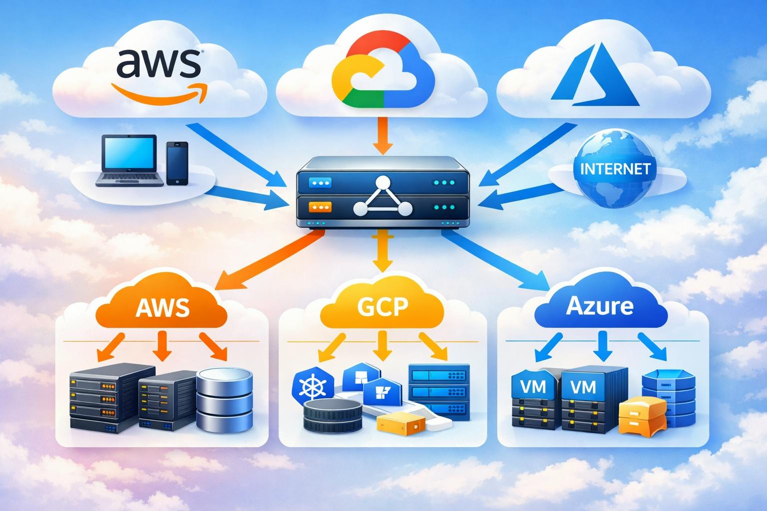
As a senior cloud engineer who has architected solutions across multiple cloud platforms, I’ve learned that choosing the right load balancer can make or break your application’s performance, scalability, and cost efficiency. This guide dives deep into the load balancing offerings from AWS, GCP, and Azure, explaining how they work internally and when to use each type.
Understanding Load Balancer Fundamentals
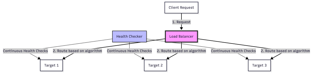
Before we dive into specific offerings, let’s understand what happens inside a load balancer. At its core, a load balancer is a reverse proxy that distributes incoming traffic across multiple backend targets based on various algorithms and health checks.
AWS Load Balancers
AWS offers four types of load balancers, each designed for specific use cases.
1. Application Load Balancer (ALB)
OSI Layer: Layer 7 (Application)
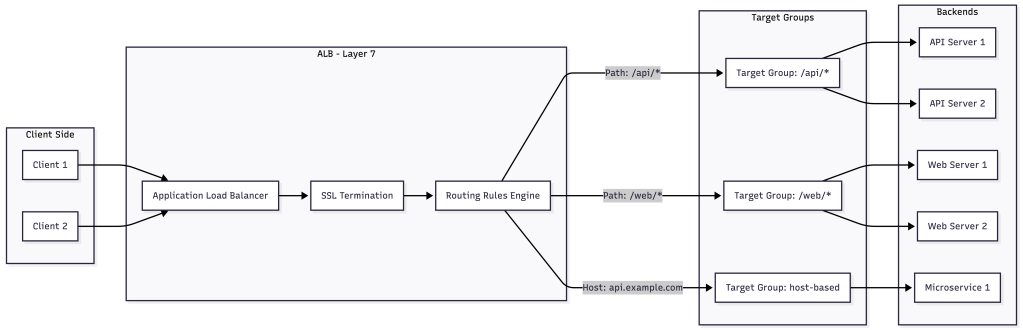
Internal Architecture: ALB operates at the HTTP/HTTPS level, parsing request headers, paths, and host information to make intelligent routing decisions. It maintains connection pooling to backend targets and handles SSL/TLS termination efficiently.
When to Use ALB:
- Modern web applications with HTTP/HTTPS traffic
- Microservices architectures requiring path-based or host-based routing
- Applications needing WebSocket support
- When you need content-based routing (headers, query strings, HTTP methods)
- Authentication integration (OIDC, SAML) at the load balancer level
- Lambda function targets
Key Features:
- Advanced request routing with multiple rules per listener
- Native integration with AWS WAF for security
- HTTP/2 and gRPC support
- Fixed response and redirect actions
- Sticky sessions with application-controlled duration
Pricing Model: Hourly rate + LCU (Load Balancer Capacity Units) based on new connections, active connections, processed bytes, and rule evaluations.
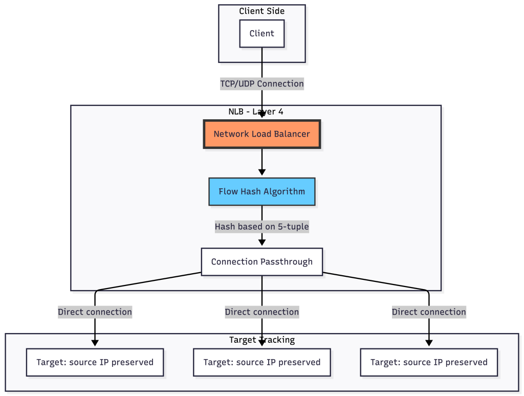
2. Network Load Balancer (NLB)
OSI Layer: Layer 4 (Transport)
Internal Architecture: NLB operates at the TCP/UDP level and uses flow hash algorithm (source IP, source port, destination IP, destination port, protocol) to route connections. It preserves source IP addresses and can handle millions of requests per second with ultra-low latency.
When to Use NLB:
- Extreme performance requirements (millions of requests/sec)
- Applications requiring static IP addresses or Elastic IPs
- TCP/UDP traffic that doesn’t need HTTP-level inspection
- When you need to preserve source IP addresses
- Applications sensitive to latency (sub-millisecond)
- Non-HTTP protocols (SMTP, FTP, game servers)
- PrivateLink endpoints
Key Features:
- Ultra-low latency and high throughput
- Static IP addresses per availability zone
- Preserves source IP address
- TLS termination with SNI support
- Zonal isolation for fault tolerance
- UDP and TCP_UDP listener support
Pricing Model: Hourly rate + NLCU (Network Load Balancer Capacity Units) based on processed bytes and connections.
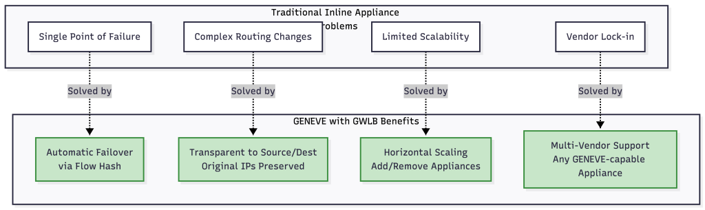
3. Gateway Load Balancer (GWLB)
OSI Layer: Layer 3 (Network)
Internal Architecture: GWLB operates using GENEVE protocol encapsulation on port 6081. It transparently passes traffic to third-party virtual appliances for inspection before forwarding to destinations.
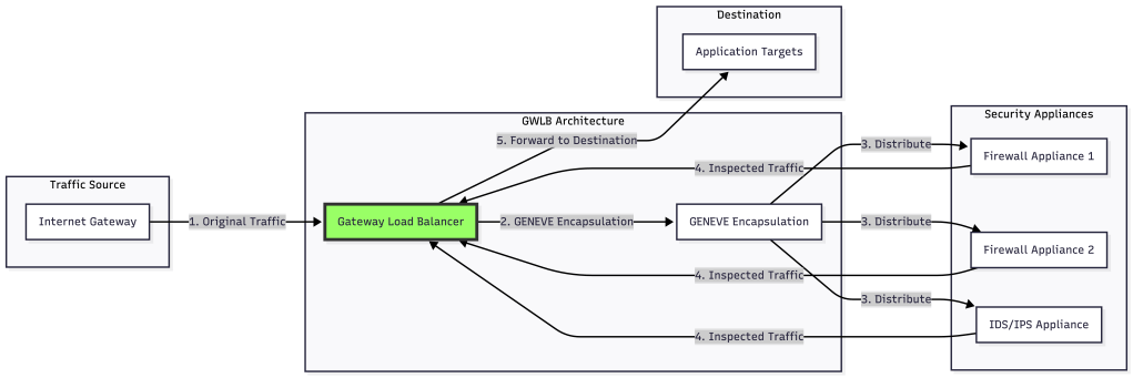
When to Use GWLB:
- Deploying third-party network virtual appliances (firewalls, IDS/IPS)
- Centralized security inspection architecture
- Traffic inspection that must be transparent to source and destination
- Scaling security appliances horizontally
- Multi-tenant security service offerings
Key Features:
- Transparent to source and destination
- Supports multiple security vendors
- Automatic scaling and health checking of appliances
- GENEVE protocol encapsulation preserves original packet information
4. Classic Load Balancer (CLB)
Status: Legacy (not recommended for new applications)
When to Use CLB: Only for existing EC2-Classic applications. Migrate to ALB or NLB for new workloads.
Google Cloud Platform Load Balancers
GCP takes a different architectural approach with its global load balancing infrastructure, offering both global and regional load balancers.
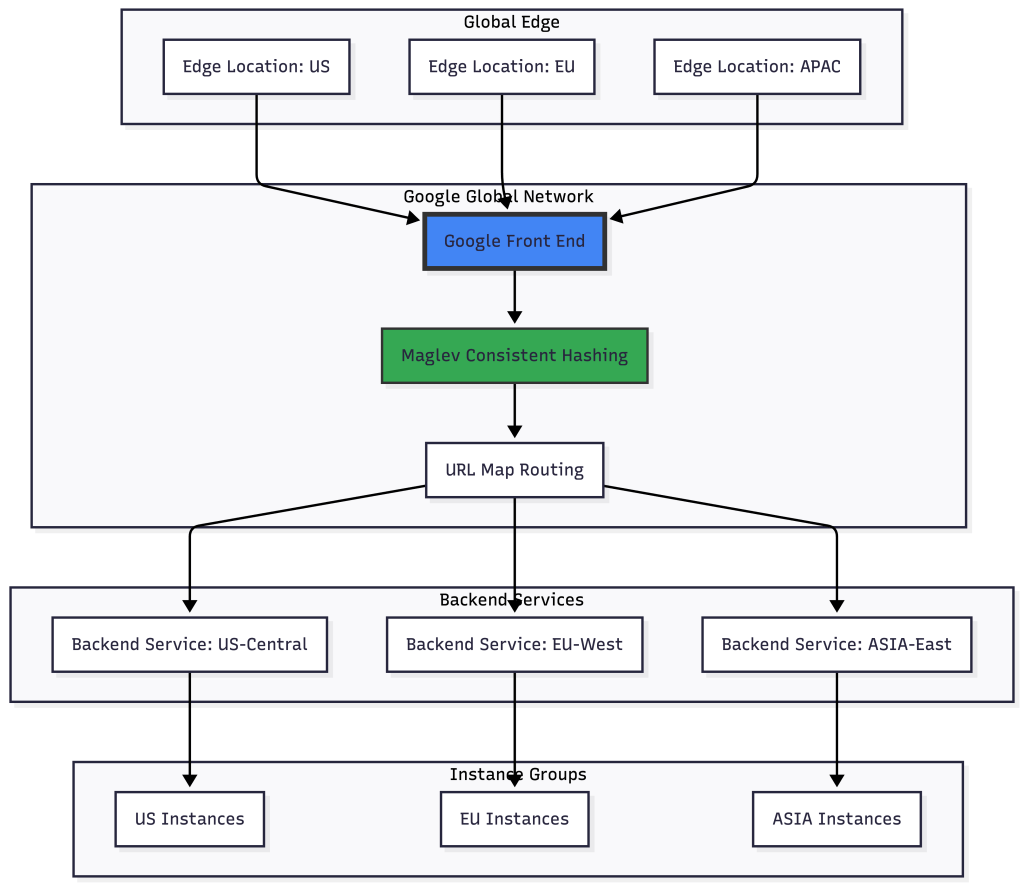
1. Global External Application Load Balancer
OSI Layer: Layer 7
Internal Architecture: Built on Google’s global network infrastructure using Andromeda (Google’s SDN stack) and Maglev (consistent hashing load balancer). Traffic enters at Google’s edge locations closest to users and is routed through their private backbone.
When to Use:
- Global applications serving users worldwide
- Need for intelligent global traffic routing
- Anycast IP for automatic DDoS mitigation
- Multi-region failover and load distribution
- SSL/TLS offloading at Google’s edge
- Applications requiring Cloud CDN integration
Key Features:
- Single global anycast IP address
- Automatic multi-region failover
- Cross-region load balancing
- Built-in Cloud Armor for DDoS protection
- HTTP/2 and QUIC protocol support
- URL map-based routing with path, host, and header matching
2. Global External Network Load Balancer
OSI Layer: Layer 4
Internal Architecture: Uses Google’s Maglev for consistent hashing across backend pools. Supports both Premium Tier (global) and Standard Tier (regional) networking.
When to Use:
- Global TCP/UDP applications
- Need for preserving source IP
- Non-HTTP(S) protocols at global scale
- Gaming servers with global distribution
- IoT applications with worldwide devices
3. Regional External Application Load Balancer
OSI Layer: Layer 7
When to Use:
- Applications confined to a single region
- Lower cost alternative when global routing isn’t needed
- Regulatory requirements for data locality
- Private RFC 1918 IP addresses for external load balancing
4. Internal Application Load Balancer
OSI Layer: Layer 7
Internal Architecture: Implemented using Google-managed Envoy-based proxies (not user-configurable), providing L7 features similar to Envoy but without direct proxy control. Fully distributed with no single point of failure.
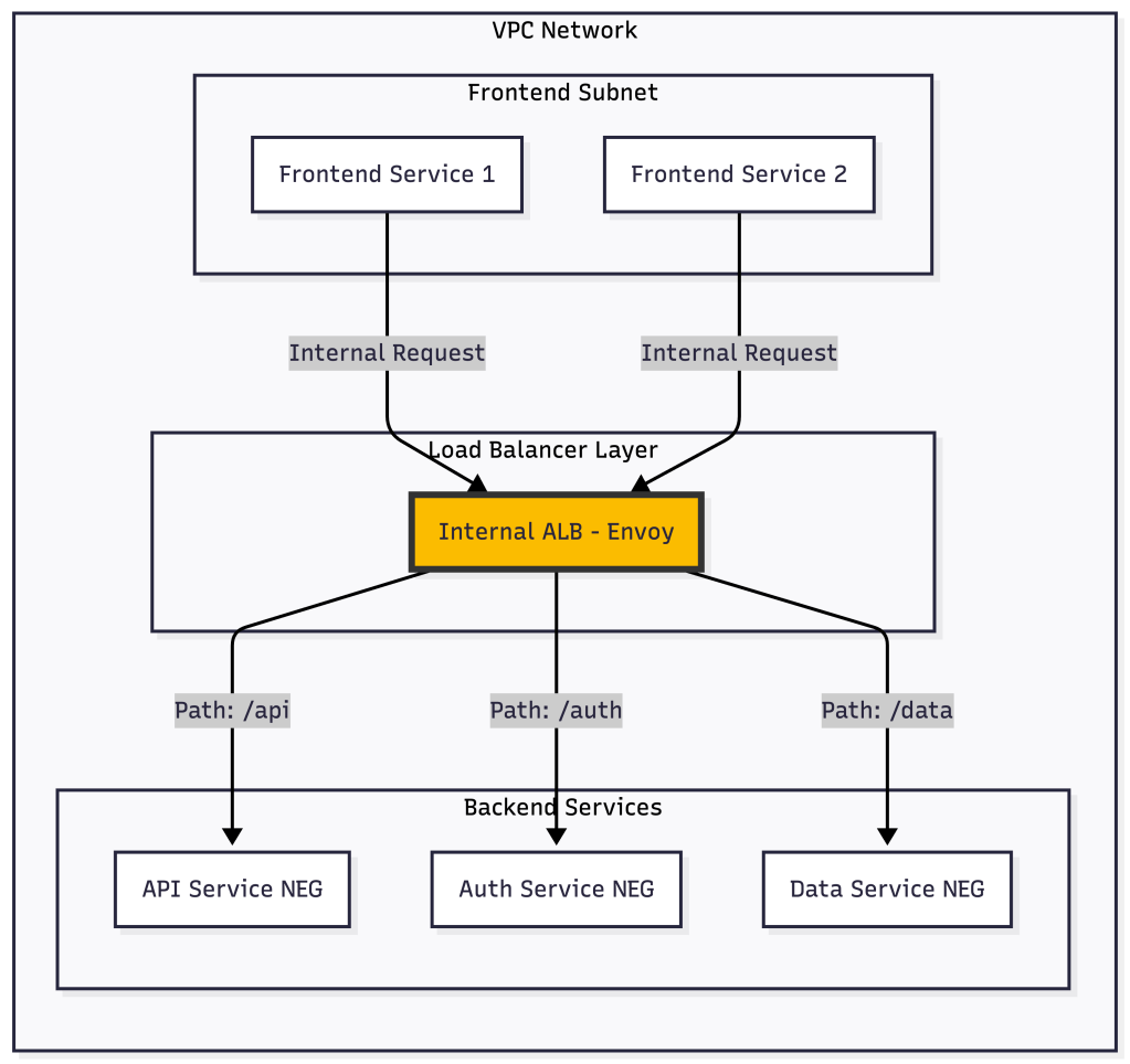
When to Use:
- Internal microservices communication
- Private service mesh without external exposure
- Supports multi-region backends when configured with global access.
- Service-to-service authentication requirements
Key Features:
- Built on Envoy proxy (same as Istio)
- Advanced traffic management (retry, timeout, circuit breaking)
- Works with GKE, Compute Engine, and Cloud Run
- Network Endpoint Groups (NEGs) for container-native load balancing
5. Internal Network Load Balancer
OSI Layer: Layer 4
When to Use:
- Internal TCP/UDP load balancing
- High-performance internal services
- Database connection pooling
- Legacy applications requiring Layer 4 balancing
Azure Load Balancers
Azure offers load balancing solutions integrated with its global network fabric and supports both PaaS and IaaS workloads.
1. Azure Application Gateway
OSI Layer: Layer 7
Internal Architecture: Regional service that acts as an Application Delivery Controller (ADC) with integrated Web Application Firewall. Uses round-robin by default with session affinity options.
When to Use:
- HTTP/HTTPS web applications
- Applications requiring Web Application Firewall
- URL-based routing and SSL termination
- Azure App Service and VM backend pools
- Private or public facing web applications
- Cookie-based session affinity requirements
Key Features:
- Integrated WAF with OWASP core rule sets
- Autoscaling with zone redundancy
- HTTP to HTTPS redirection
- Custom error pages
- URL path-based and multi-site routing
- Connection draining
- WebSocket and HTTP/2 support
SKUs: Standard_v2 and WAF_v2 (v1 is being retired)
2. Azure Load Balancer
OSI Layer: Layer 4
Internal Architecture: Zone-redundant by default in regions that support availability zones. Uses 5-tuple hash (source IP, source port, destination IP, destination port, protocol) for distribution.
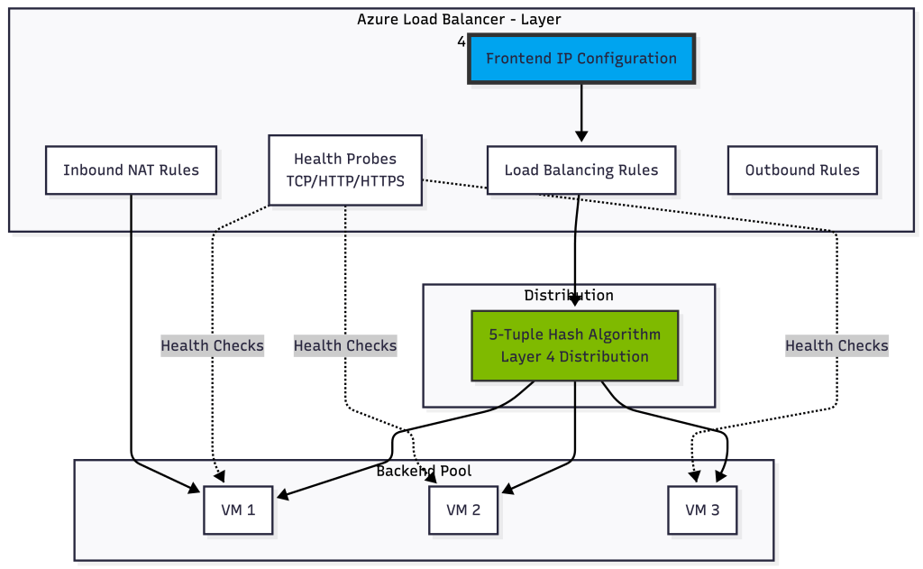
When to Use:
- Internal or external TCP/UDP traffic
- High availability for VM-based applications
- Port forwarding scenarios
- Hybrid scenarios with on-premises connectivity
- Low-latency, high-throughput applications
- All TCP/UDP protocols including RDP and SSH
Key Features:
- Zone-redundant and zonal deployments
- Internal and external load balancers
- High availability ports for NVAs
- TCP and UDP protocol support
- Floating IP for SQL AlwaysOn
- Outbound connectivity management
- HA Ports for load balancing all ports
SKUs: Basic (being retired) and Standard
3. Azure Front Door
OSI Layer: Layer 7 (Global)
Internal Architecture: Operates at Microsoft’s global edge network with over 185 edge locations. Uses anycast protocol with split TCP and HTTP acceleration.
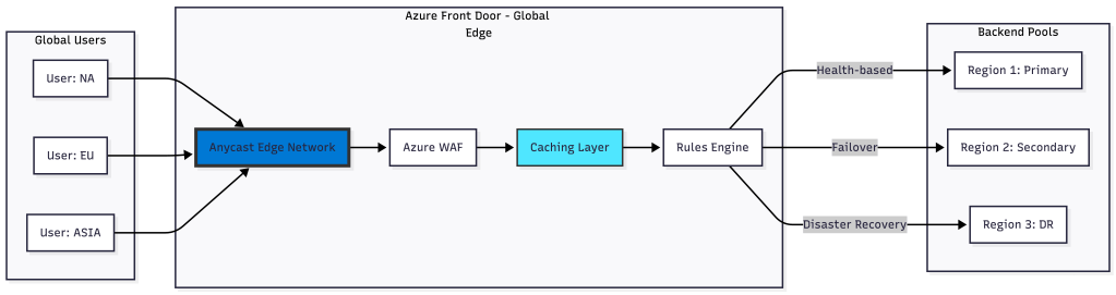
When to Use:
- Global web applications requiring acceleration
- Multi-region applications with automatic failover
- Microservices requiring global routing
- Applications needing global DDoS protection
- Content delivery and caching requirements
- URL-based routing across regions
Key Features:
- Global HTTP load balancing and acceleration
- SSL offload at edge locations
- Path-based routing and URL rewrite
- Integrated CDN functionality
- Real-time metrics and alerting
- Rules engine for custom routing logic
- Private Link support to origin
Tiers: Standard and Premium (includes enhanced security features)
4. Azure Traffic Manager
OSI Layer: DNS level (not a proxy)
Internal Architecture: DNS-based traffic routing service that responds to DNS queries with the IP of the optimal endpoint based on routing method.
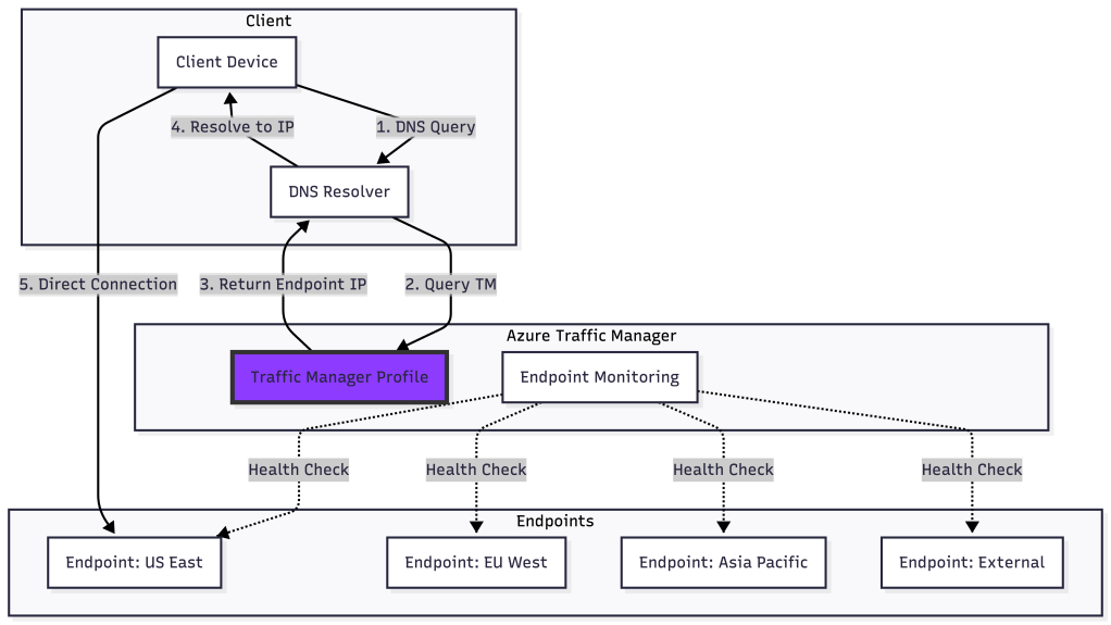
When to Use:
- DNS-level global traffic distribution
- Routing based on geographic location
- Weighted traffic distribution for A/B testing
- Priority-based failover scenarios
- Low cost global routing solution
- Hybrid cloud and on-premises endpoints
Routing Methods:
- Priority: Failover to backup endpoints
- Weighted: Distribute traffic by percentage
- Performance: Route to lowest latency endpoint
- Geographic: Route based on DNS query origin
- Multivalue: Return multiple healthy endpoints
- Subnet: Map specific IP ranges to endpoints
Important Limitation: Traffic Manager only provides DNS resolution, not proxy functionality. Clients connect directly to endpoints after DNS resolution.
Comparison Matrix
Layer 7 (Application) Load Balancers
|
Feature |
AWS ALB |
GCP Global ALB |
GCP Regional ALB |
GCP Internal ALB |
Azure App Gateway |
Azure Front Door |
|---|---|---|---|---|---|---|
|
Scope |
Regional |
Global |
Regional |
Regional (Internal) |
Regional |
Global |
|
SSL Termination |
✓ |
✓ |
✓ |
✓ |
✓ |
✓ |
|
Path Routing |
✓ |
✓ |
✓ |
✓ |
✓ |
✓ |
|
Host Routing |
✓ |
✓ |
✓ |
✓ |
✓ |
✓ |
|
Integrated WAF |
✓ |
✓ (Cloud Armor) |
✓ (Cloud Armor) |
✗ |
✓ (OWASP) |
✓ (Premium tier) |
|
HTTP/2 & gRPC |
✓ |
✓ |
✓ |
✓ |
✓ |
✓ |
|
WebSocket |
✓ |
✓ |
✓ |
✓ |
✓ |
✓ |
|
Serverless Support |
✓ (Lambda) |
✓ (Cloud Run) |
✓ (Cloud Run) |
✓ (Cloud Run) |
✓ (Functions) |
✓ (Functions) |
|
Built-in CDN |
✗ |
✓ |
✗ |
✗ |
✗ |
✓ |
|
Global Anycast IP |
✗ |
✓ |
✗ |
✗ |
✗ |
✓ |
|
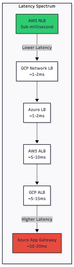
Typical Latency |
5-10ms |
5-15ms |
5-10ms |
5-10ms |
10-20ms |
10-30ms* |
|
Best For |
Microservices, APIs |
Global web apps |
Regional web apps |
Internal services |
Web + WAF |
Global CDN + LB |
*Varies by user proximity to edge
Disclaimer: Latency figures are illustrative order-of-magnitude estimates observed in typical internet-facing deployments; actual latency varies significantly by region, traffic path, and backend proximity.
Layer 4 (Transport) Load Balancers
|
Feature |
AWS NLB |
GCP Global NLB |
GCP Internal NLB |
Azure Load Balancer |
|---|---|---|---|---|
|
Scope |
Regional |
Global |
Regional (Internal) |
Regional |
|
Protocol |
TCP/UDP/TLS |
TCP/UDP |
TCP/UDP |
TCP/UDP |
|
Static IP |
✓ |
✓ (Anycast) |
✓ |
✓ |
|
Preserve Source IP |
✓ |
✓ |
✓ |
✓ |
|
TLS Termination |
✓ |
✓ |
✗ |
✗ |
|
WebSocket-compatible (TCP pass-through) |
✓ |
✓ |
✓ |
✓ |
|
Connection Handling |
Millions/sec |
Millions/sec |
High throughput |
High throughput |
|
Typical Latency |
<1ms |
1-2ms |
1-2ms |
~1–5ms (region and topology dependent) |
|
Zone Redundant |
✓ |
✓ |
✓ |
✓ |
|
Best For |
High performance, gaming, IoT |
Global TCP/UDP apps |
Internal TCP/UDP |
VM load balancing, RDP/SSH |
Disclaimer: Latency figures are illustrative order-of-magnitude estimates observed in typical internet-facing deployments; actual latency varies significantly by region, traffic path, and backend proximity.
NOTE: Azure Load Balancer – TLS termination requires Application Gateway or Front Door.
Specialized Load Balancers
|
Feature |
AWS GWLB |
Azure Traffic Manager |
|---|---|---|
|
Type |
Layer 3 Gateway |
DNS-based routing |
|
Primary Use |
Security appliance insertion |
Global DNS routing |
|
Protocol |
GENEVE encapsulation (UDP 6081) |
DNS resolution |
|
Routing Method |
Flow hash to appliances |
Priority, Weighted, Geographic, Performance |
|
Preserves Traffic |
✓ (Transparent) |
N/A (DNS only) |
|
Integrated WAF |
✗ (Routes to 3rd party) |
✗ |
|
Failover |
Automatic (via health checks) |
Automatic (via health checks) |
|
Typical Latency |
1-3ms |
DNS resolution only |
|
Best For |
Centralized security inspection, IDS/IPS |
Low-cost global failover, hybrid cloud |
Disclaimer: Latency figures are illustrative order-of-magnitude estimates observed in typical internet-facing deployments; actual latency varies significantly by region, traffic path, and backend proximity.
Quick Decision Guide
Choose Layer 7 (ALB/App Gateway/Front Door) when:
- HTTP/HTTPS traffic
- Need path/host-based routing
- SSL termination required
- WAF protection needed
- Microservices architecture
Choose Layer 4 (NLB/Load Balancer) when:
- Extreme performance needed (<1ms latency)
- Non-HTTP protocols (gaming, databases, SMTP)
- Need to preserve source IP
- Static IP addresses required
- Millions of requests per second
Choose Specialized (GWLB/Traffic Manager) when:
- GWLB: Transparent security inspection with 3rd party appliances
- Traffic Manager: DNS-based global routing at lowest cost
Provider Strengths Summary
AWS:
- Most comprehensive LB portfolio (4 types)
- Best sub-millisecond latency (NLB)
- Unique GENEVE-based security integration (GWLB)
- Strong serverless integration
GCP:
- True global load balancing with anycast
- Maglev consistent hashing (minimal disruption)
- Envoy-based internal ALB (service mesh ready)
- Best for global applications
Azure:
- Most diverse offerings (4 LB types + Traffic Manager)
- Front Door combines CDN + LB + WAF
- Mature WAF with OWASP rule sets
- Strong hybrid cloud support
- Traffic Manager for cost-effective DNS routing
Performance Characteristics
Decision Framework
Use Case: E-commerce Website
Requirements: Global presence, WAF protection, path-based routing, SSL termination
Recommended Solution:
- AWS: CloudFront + ALB per region
- GCP: Global External Application Load Balancer + Cloud Armor
- Azure: Azure Front Door Premium
Use Case: Real-time Gaming
Requirements: Ultra-low latency, UDP support, static IPs, preserve source IP
Recommended Solution:
- AWS: Network Load Balancer
- GCP: Global External Network Load Balancer
- Azure: Azure Load Balancer (Standard)
Use Case: Internal Microservices
Requirements: Service mesh, advanced routing, circuit breaking, internal only
Recommended Solution:
- AWS: ALB with Target Groups
- GCP: Internal Application Load Balancer (Envoy-based)
- Azure: Application Gateway (internal) or API Management
Use Case: Hybrid Cloud Application
Requirements: On-premises and cloud, DNS-based routing, health monitoring
Recommended Solution:
- AWS: Route 53 + NLB
- GCP: Cloud DNS + Global Load Balancer
- Azure: Traffic Manager + Azure Load Balancer
Cost Optimization Tips
- Right-size your load balancer: Don’t use Application Load Balancers for simple TCP traffic; Network Load Balancers are often cheaper and more performant.
- Minimize cross-region data transfer: Use regional load balancers when global distribution isn’t required to avoid cross-region charges.
- Leverage autoscaling: Configure proper scaling policies to avoid over-provisioning during low-traffic periods.
- Use connection pooling: For HTTP traffic, connection pooling reduces overhead and improves efficiency.
- Monitor your LCUs/NLCUs: In AWS, understanding what drives your capacity unit consumption helps optimize costs.
- Consider Traffic Manager for Azure: For simple DNS-based routing, Traffic Manager is significantly cheaper than Front Door or Application Gateway.
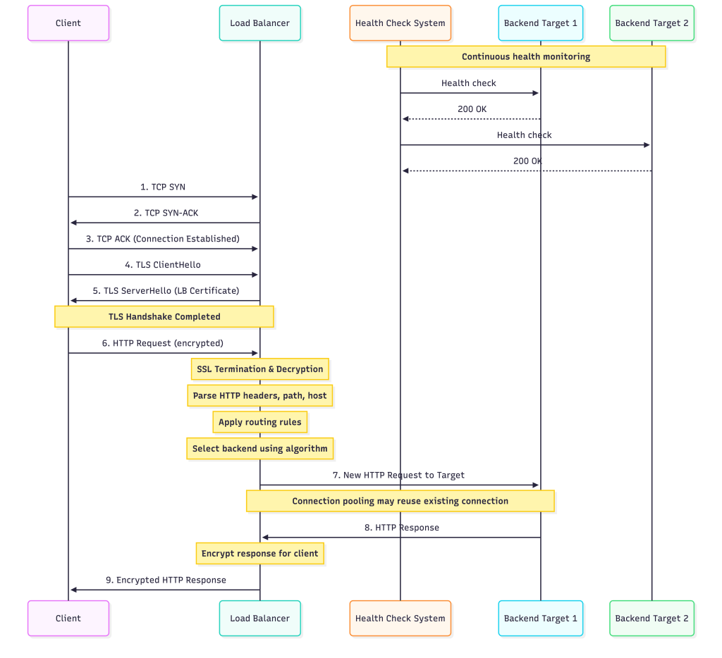
Internal Working: Connection Flow Deep Dive
Let’s examine what happens internally when a request hits a Layer 7 load balancer:
Monitoring and Observability
Each cloud provider offers comprehensive metrics:
AWS CloudWatch Metrics:
- TargetResponseTime: Latency from load balancer to target
- HealthyHostCount/UnHealthyHostCount: Target health status
- RequestCount: Total requests processed
- ActiveConnectionCount: Current connections
- ConsumedLCUs: Capacity unit consumption
GCP Cloud Monitoring:
- request_count: Total requests handled
- backend_latencies: Latency to backends
- total_latencies: End-to-end latency including load balancer
- backend_request_count: Requests per backend
Azure Monitor:
- ByteCount: Data processed
- PacketCount: Packets processed
- HealthProbeStatus: Backend health
- DipAvailability: Backend availability percentage
Final Recommendations
- Start with managed services: All three providers offer robust managed load balancing. Don’t build your own unless you have very specific requirements.
- Understand the OSI layer: Match your load balancer to your traffic type. Layer 7 for HTTP/HTTPS, Layer 4 for other TCP/UDP.
- Plan for global scale: If you’re building for a global audience, GCP’s global load balancer or Azure Front Door provides the best out-of-the-box experience.
- Security first: Always enable WAF protection for internet-facing applications using AWS WAF, Cloud Armor, or Azure WAF.
- Monitor everything: Set up comprehensive monitoring and alerting on health check failures, latency increases, and capacity limits.
- Test failover: Regularly test your disaster recovery and failover scenarios to ensure load balancers route traffic correctly when backends fail.
The landscape of cloud load balancers continues to evolve with new features and capabilities. As a senior engineer, staying current with these offerings and understanding their internal architecture allows you to make informed decisions that balance performance, cost, and operational complexity.
Appendix
Flow Hash Algorithm
What is Flow Hash?
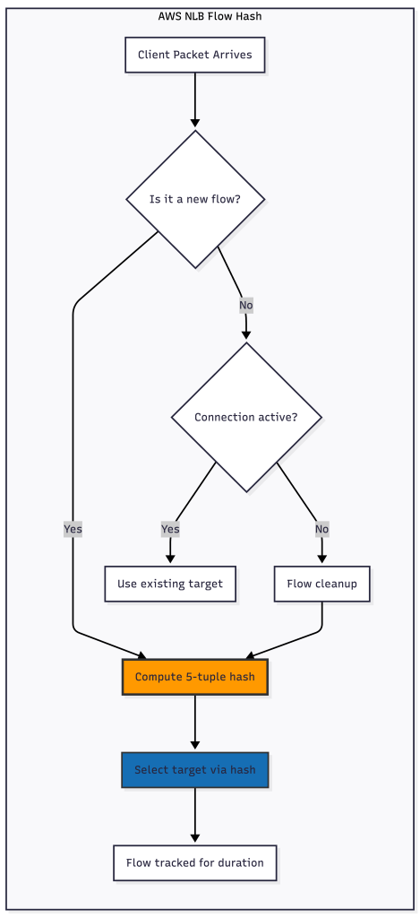
Flow hash is a deterministic algorithm used by Layer 4 load balancers to distribute connections across backend servers. The key principle is that packets belonging to the same connection (or “flow”) always route to the same backend server, ensuring session persistence without requiring the load balancer to maintain state.
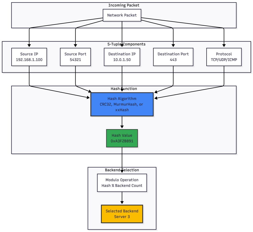
The 5-Tuple Hash
The most common flow hash implementation uses a 5-tuple hash, which creates a unique identifier from five components of each packet:
How Flow Hash Works Step-by-Step
Step 1: Extract the 5-Tuple
When a packet arrives, the load balancer extracts:
- Source IP Address:
192.168.1.100 - Source Port:
54321 - Destination IP Address:
10.0.1.50 - Destination Port:
443(HTTPS) - Protocol:
6(TCP)
Step 2: Compute the Hash
These five values are concatenated and passed through a hash function:
Input: 192.168.1.100:54321 -> 10.0.1.50:443 (TCP) Hash Function: CRC32 or similar Output: 2746089617 (0xA3F2B891 in hex)
Step 3: Select Backend Using Modulo
If we have 4 backend servers, we use modulo operation:
Backend Index = Hash Value % Number of Backends
Backend Index = 2746089617 % 4 = 1
Therefore, this connection routes to Backend Server 1.
Connection Flow with Hash Consistency
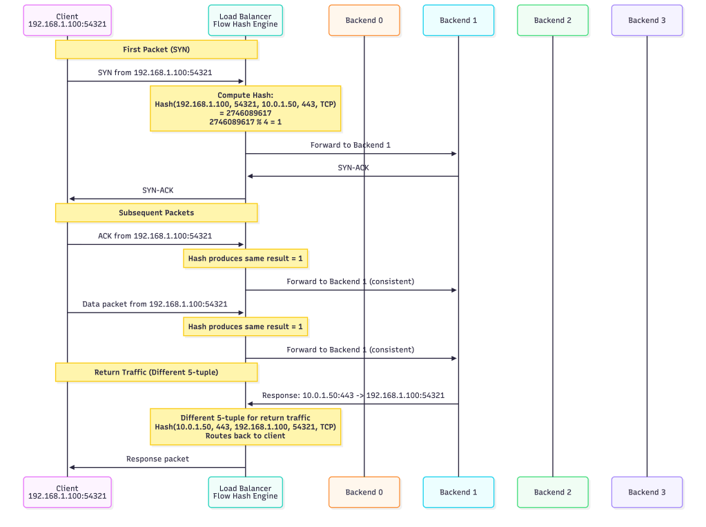
Advantages of Flow Hash
- Stateless: Does not maintain application-layer session state; tracks flows at the transport layer for consistency.
- Fast: Hash computation is extremely fast (nanoseconds)
- Scalable: Can handle millions of flows without memory overhead
- Session Persistence: All packets in a flow go to the same backend
- Symmetric: Can be used for both directions if needed
Challenges and Solutions
Problem 1: Backend Changes
When backends are added or removed, many flows get remapped:
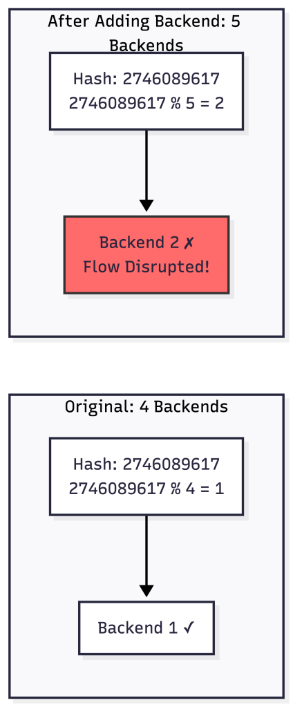
Solution: Consistent Hashing
Google’s Maglev and other modern load balancers use consistent hashing to minimize flow disruption:
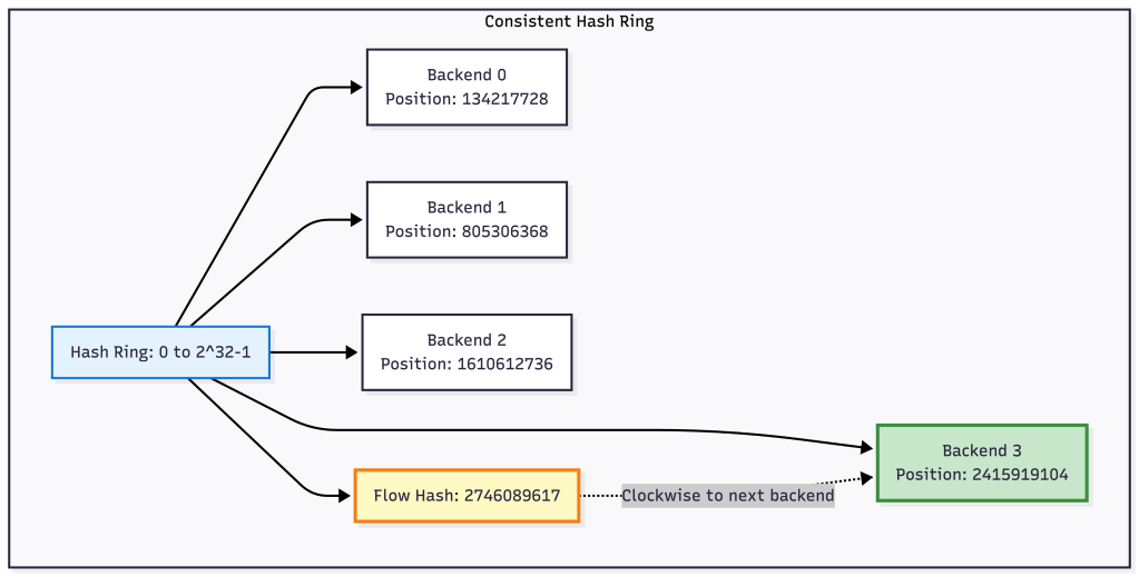
With consistent hashing, only flows near the removed/added backend are affected, not all flows.
Problem 2: Uneven Distribution
Simple modulo can create uneven distribution with certain hash functions:
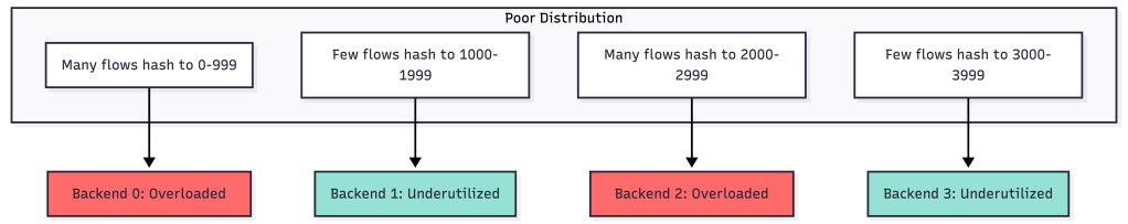
Solution: Use high-quality hash functions like MurmurHash3 or xxHash that provide uniform distribution.
Real-World Example: AWS NLB
AWS Network Load Balancer uses flow hash with these characteristics:
Variations of Flow Hash
3-Tuple Hash (Less common):
- Source IP
- Destination IP
- Protocol
Use case: When you want all connections from a client to go to the same backend regardless of port.
2-Tuple Hash:
- Source IP
- Destination IP
Use case: Geographic affinity or client-based routing.
GENEVE Protocol Encapsulation
What is GENEVE?
GENEVE (Generic Network Virtualization Encapsulation) is a tunneling protocol designed for network virtualization. It’s the successor to VXLAN and NVGRE, providing a flexible framework for encapsulating network packets.
GENEVE is used by AWS Gateway Load Balancer (GWLB) to transparently route traffic through security appliances like firewalls, IDS/IPS systems, and network packet brokers.
GENEVE Packet Structure

GENEVE Header Format
 0                   1                   2                   3
 0 1 2 3 4 5 6 7 8 9 0 1 2 3 4 5 6 7 8 9 0 1 2 3 4 5 6 7 8 9 0 1
+-+-+-+-+-+-+-+-+-+-+-+-+-+-+-+-+-+-+-+-+-+-+-+-+-+-+-+-+-+-+-+-+
|Ver|  Opt Len  |O|C|    Rsvd.  |          Protocol Type        |
+-+-+-+-+-+-+-+-+-+-+-+-+-+-+-+-+-+-+-+-+-+-+-+-+-+-+-+-+-+-+-+-+
|        Virtual Network Identifier (VNI)       |    Reserved   |
+-+-+-+-+-+-+-+-+-+-+-+-+-+-+-+-+-+-+-+-+-+-+-+-+-+-+-+-+-+-+-+-+
|                    Variable Length Options                    |
+-+-+-+-+-+-+-+-+-+-+-+-+-+-+-+-+-+-+-+-+-+-+-+-+-+-+-+-+-+-+-+-+
Field Breakdown:
- Ver (2 bits): Version = 0
- Opt Len (6 bits): Length of options in 4-byte words
- O (1 bit): OAM packet flag
- C (1 bit): Critical options present
- Protocol Type (16 bits): Inner protocol (0x6558 for Ethernet)
- VNI (24 bits): Virtual Network Identifier
- Options: Variable length metadata
How AWS GWLB Uses GENEVE
GENEVE Encapsulation Example
Original Packet (HTTP Request):
Ethernet: [Src MAC: Client] [Dst MAC: Gateway]
IP:       [Src: 203.0.113.50] [Dst: 10.0.2.50]
TCP:      [Src Port: 54321] [Dst Port: 80]
Data:     GET /index.html HTTP/1.1...
After GENEVE Encapsulation by GWLB:
Outer Ethernet: [Src MAC: GWLB ENI] [Dst MAC: Firewall ENI]
Outer IP:       [Src: 10.0.0.50] [Dst: 10.0.1.100]
Outer UDP:      [Src Port: Random] [Dst Port: 6081]
GENEVE Header:  [VNI: 12345] [Protocol: Ethernet]
Inner Ethernet: [Src MAC: Client] [Dst MAC: Gateway]
Inner IP:       [Src: 203.0.113.50] [Dst: 10.0.2.50]
Inner TCP:      [Src Port: 54321] [Dst Port: 80]
Inner Data:     GET /index.html HTTP/1.1...
Why GENEVE for Security Appliances?
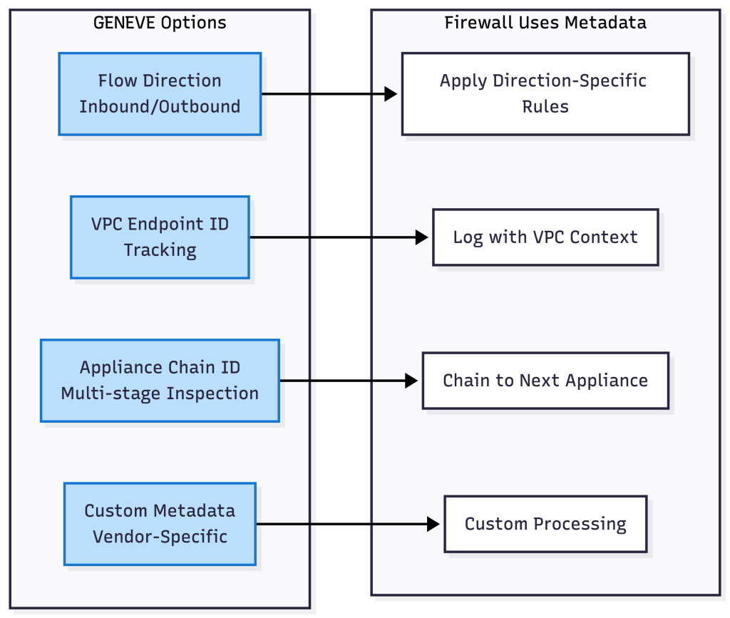
GENEVE Options and Metadata
GENEVE supports variable-length options for carrying metadata:
GENEVE vs VXLAN vs GRE
|
Feature |
GENEVE |
VXLAN |
GRE |
|---|---|---|---|
|
Encapsulation Protocol |
UDP (Port 6081) |
UDP (Port 4789) |
IP Protocol 47 |
|
Header Overhead |
8 bytes + options |
8 bytes fixed |
4+ bytes |
|
Flexibility |
Variable options |
Fixed header |
Limited options |
|
VNI/VSID Size |
24 bits |
24 bits |
32 bits (key) |
|
Metadata Support |
Extensive via options |
Limited |
Very limited |
|
Industry Adoption |
Growing (AWS, VMware) |
Widespread |
Legacy |
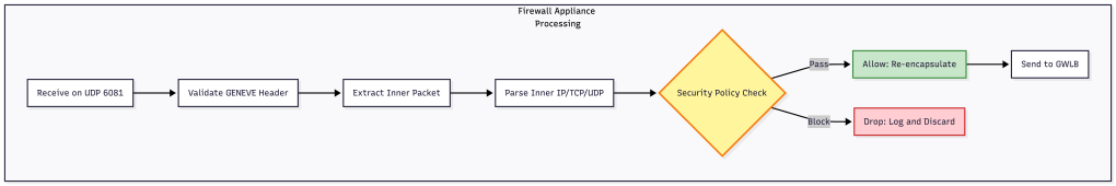
Security Appliance Configuration
For an appliance to work with GWLB, it must:
- Listen on UDP port 6081 for GENEVE traffic
- Decapsulate GENEVE headers to access inner packet
- Inspect the inner packet according to security policies
- Re-encapsulate the packet with GENEVE
- Send back to GWLB at the source IP of the GENEVE packet
Example Packet Flow in Appliance:
Performance Considerations
Overhead Analysis:
Original Packet: 1500 bytes
  ├─ Ethernet: 14 bytes
  ├─ IP: 20 bytes
  ├─ TCP: 20 bytes
  └─ Data: 1446 bytes

GENEVE Encapsulated: 1558 bytes
  ├─ Outer Ethernet: 14 bytes
  ├─ Outer IP: 20 bytes
  ├─ Outer UDP: 8 bytes
  ├─ GENEVE: 16 bytes (8 base + 8 options)
  └─ Inner Original Packet: 1500 bytes

Overhead: 58 bytes (3.9%)
Throughput Impact:
- GENEVE encap/decap: ~5-10 microseconds per packet
- Hardware offload available on modern NICs
- Appliances can process 10-100 Gbps with proper tuning
Debugging GENEVE
Capture GENEVE traffic with tcpdump:
# Capture GENEVE packets
tcpdump -i eth0 udp port 6081 -vvv -X

# Decode GENEVE with specific filter
tcpdump -i eth0 'udp port 6081' -vvv -XX
Sample GENEVE packet capture:
IP 10.0.0.50.54321 > 10.0.1.100.6081: UDP, length 1524
    0x0000:  4500 060c 1234 0000 4011 xxxx 0a00 0032  E....4..@......2
    0x0010:  0a00 0164 d431 17c1 05f8 xxxx 0000 6558  ...d.1........eX
    0x0020:  0030 3900 0000 0000 ... (GENEVE header)
    0x0030:  ... (Inner Ethernet frame)
Real-World Use Case: Centralized Egress Filtering
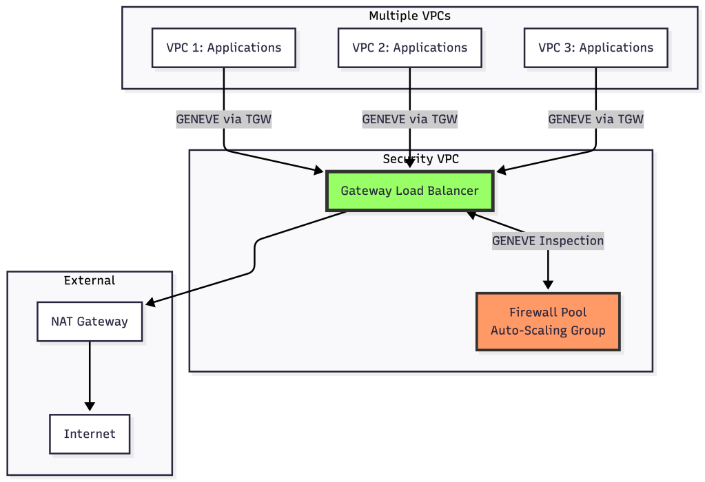
In this architecture:
- All VPCs route traffic to GWLB via Transit Gateway
- GWLB encapsulates with GENEVE and distributes to firewall pool using flow hash
- Firewalls inspect and return to GWLB
- GWLB decapsulates and routes to NAT Gateway/Internet
- Scaling firewalls doesn’t disrupt existing flows (consistent hashing)
Summary
Flow Hash Algorithm:
- Deterministic load distribution using packet 5-tuple
- Stateless and extremely fast
- Ensures session persistence
- Modern implementations use consistent hashing for minimal disruption
GENEVE Protocol:
- Flexible tunneling for network virtualization
- Preserves original packet information completely
- Enables transparent security appliance insertion
- Supports rich metadata via variable options
- AWS GWLB’s foundation for scalable security architectures
Both technologies work together in systems like AWS GWLB: flow hash ensures consistent routing to appliances, while GENEVE enables transparent inspection without breaking application layer contexts.
Have questions about specific load balancer configurations or migration strategies? Feel free to reach out or leave a comment below.
[story continues]
tags