Table of Links
1.2. Basics of neural networks
1.3. About the entropy of direct PINN methods
1.4. Organization of the paper
-
Non-diffusive neural network solver for one dimensional scalar HCLs
2.2. Arbitrary number of shock waves
2.5. Non-diffusive neural network solver for one dimensional systems of CLs
-
Gradient descent algorithm and efficient implementation
-
Numerics
4.1. Practical implementations
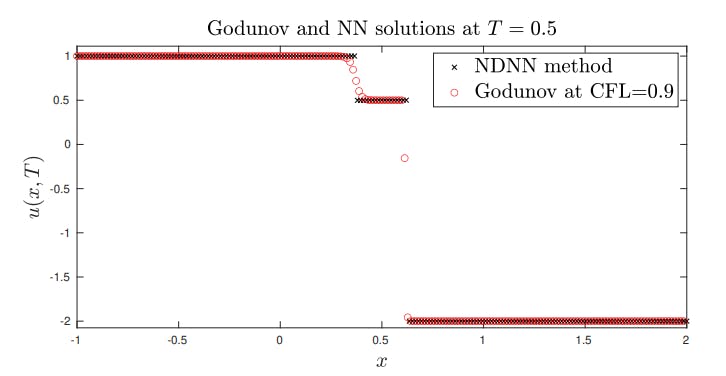
4.2. Basic tests and convergence for 1 and 2 shock wave problems
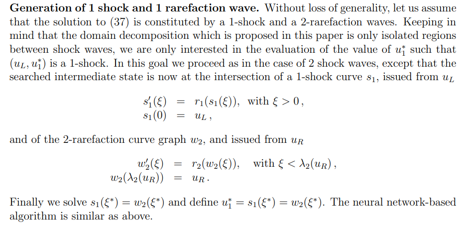
2.3. Shock wave generation
So far we have not discussed the generation of shock waves within a given domain. Interestingly the method developed above for pre-existing shock waves can be applied directly for the generation of shock waves in a given subdomain. In order to explain the principle of the approach, we simply consider one space-time domain Ω × [0, T]. We initially assume that: i) u0 is a smooth function, and ii) at time t ∗ ∈ (0, T) a shock is generated in x ∗ ∈ Ω, and the corresponding DL is defined by γ : t 7→ γ(t) for t ∈ [t ∗ , T].
Although t ∗ could be analytically estimated from −1/ minx f ′ (u0(x)), our algorithm does not require a priori the knowledge of t ∗ and x ∗ . The only required information is the fact that a shock will be generated which can again be deduced by the study of the variations of f ′ (u0).
Unlike the framework in Sections 2.1 and 2.2, here we cannot initially specify the position of the DL. However proceed here using a similar approach. Let x0 ∈ Ω be such that γ can be extended as a smooth curve in [0, T], still denoted by γ, with γ(0) = x0. Without loss of generality we may assume x0 = 0. Then we proceed exactly as in Section 2.1, with one network n representing the DL, and N± the solutions on each side of n. We define t ∗ = max{t ∈ (0, T], N+(n(t), t) = N−(n(t), t)}. Note that for t < t∗ we have N+(n(t), t) = N−(n(t), t), and the curve {n(t), t ∈ [0, t∗ )} does not have any significant meaning
2.4. Shock wave interaction
As described above, for D pre-existing shock waves we decompose the global domain in D + 1 subdomains. So far we have not considered shock wave interactions leading to a new shock wave, which reduces by one the total number of shock waves for each shock interaction.
2.5. Non-diffusive neural network solver for one dimensional systems of CLs
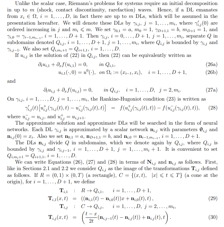
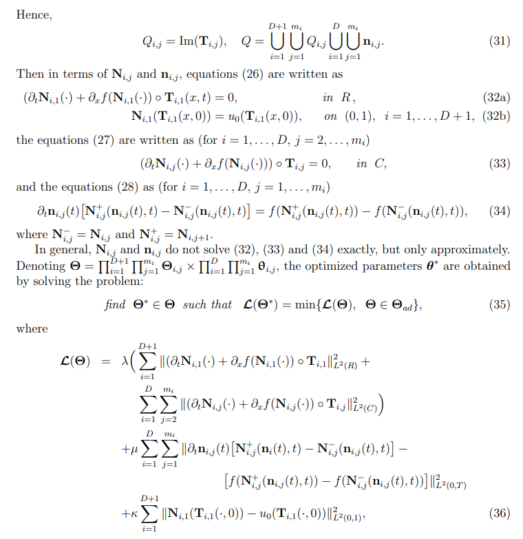
for some positive subdomain-independent parameters λ, µ and κ. Notice that when the considered IVP problems involve cones/subdomains of “very different” sizes, the choice of the hyper-parameters may be taken subdomain-dependent. This question was not investigated in this paper. If mi = 1 for all i, then the problem (11), with L given by (36), is no different from the scalar case, except that (36) involves the evaluation of norms for vector valued functions.
If Θ∗ is the solution of the problem (35), then the approximates of γi,j and of the solution u in each Qi,j is computed similarly as in Section 2.2.
2.6. Efficient initial wave decomposition
In this section we present an efficient initial wave decomposition for a Rieman problem which can be used to solve the problem (22).The idea is to solve a Riemann problem for t small, and once the states are identified we use NDNN method. Here we propose an efficient neural network based approach for the initial wave decomposition, which can easily be combined with the NDNN method. We first recall some general principles on the existence of at most m curves connecting two constant states uL and uR in the phase space. We then propose a neural network approach for constructing the rarefaction and shock curves as well as their intersection.
2.6.1. Initial wave decomposition for arbitrary m
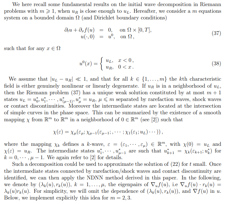
2.6.2. Initial wave decomposition for 2 equation systems (m = 2, µ = 2)
We detail the computation of the intermediate state via the construction and intersection of the shock curves (Hugoniot loci) in the phase-plane (u1, u2). Let us recall that k-shock curves are defined as the following integral curves with k = 1, 2, see [2, 6]
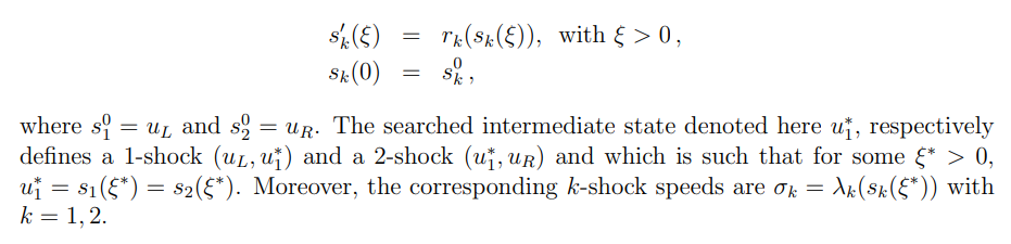
Following is the neural network strategy,
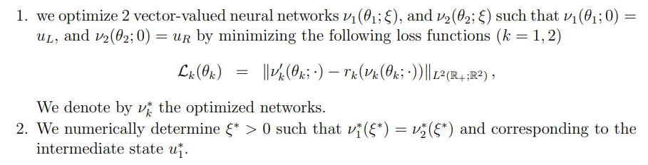
Once these intermediate waves identified, we can use them as initial condition for NDNN method.
2.6.3. Initial wave decomposition for 3 equation systems (m = 3, µ = 3)
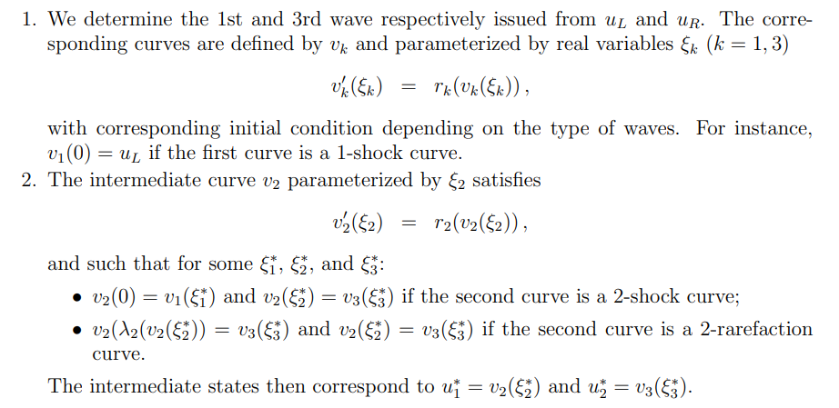
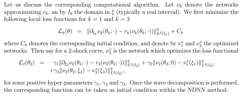
The additional difficulty compared to the case m = 2, is that the starting and ending states connected by the 2-wave are both unknown. We then propose the following approach.
Authors:
(1) Emmanuel LORIN, School of Mathematics and Statistics, Carleton University, Ottawa, Canada, K1S 5B6 and Centre de Recherches Mathematiques, Universit´e de Montr´eal, Montreal, Canada, H3T 1J4 (elorin@math.carleton.ca);
(2) Arian NOVRUZI, a Corresponding Author from Department of Mathematics and Statistics, University of Ottawa, Ottawa, ON K1N 6N5, Canada (novruzi@uottawa.ca).
This paper is
[story continues]
tags