New AI Method PreCorrector Solves Complex Diffusion Problems Faster Than Ever

Table of Links

Abstract and 1 Introduction

2 Neural design of preconditioner

3 Learn correction for ILU and 3.1 Graph neural network with preserving sparsity pattern

3.2 PreCorrector

4 Dataset

5 Experiments

5.1 Experiment environment and 5.2 Comparison with classical preconditioners

5.3 Loss function

5.4 Generalization to different grids and datasets

6 Related work

7 Conclusion and further work, and References

Appendix

3.2 PreCorrector

Instead of passing left-hand side matrix A as an input to GNN (1), we propose: (i) to pass L from IC decomposition to the GNN and (ii) to train GNN to predict a correction for this decomposition (Figure 1). We name our approach as PreCorrector (Preconditioner Corrector):

The correction coefficient α is also a learning parameter that is updated during gradient descent training. At the beginning of training, we set α = 0 to ensure that the first gradient updates come from pure IC factorization. Since we already start with a good initial guess, we observed that pinning the diagonal is redundant and limits the PreCorrector training. Moreover, GNN in (6) takes as input the lower-triangular matrix L from IC instead of A, so we are not anchored to a single specific sparse pattern of A and we can: (i) omit half of the graph and speed up the training process and (ii) use different sparsity patterns. In experiment section we show that the proposed approach with input L from IC(0) and ICt(1) indeed produce better preconditioners compared to classical IC(0) and ICt(1).

4 Dataset

We want to validate our approach on the data that addresses real-world problems. We consider a 2D diffusion equation:

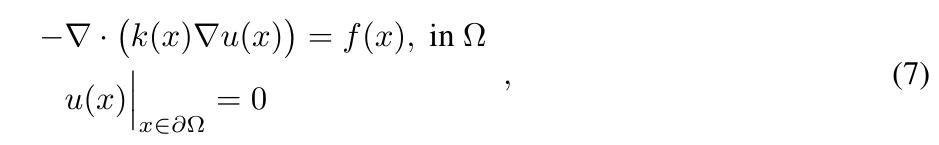
where k(x) is a diffusion coefficient, u(x) is a solution and f(x) is a forcing term.

The diffusion equation is chosen because of its frequent appearance in many engineering applications, such as: composite modeling Carr and Turner [2016], geophysical surveys Oristaglio and Hohmann [1984], fluid flow modeling Muravleva et al. [2021]. In these cases, the coefficient functions are discontinuous, i.e. they change rapidly within neighbouring cells. An example of this is the flow of fluids of different viscosities.

We propose to measure the complexity of the dataset by contrast of the coefficient function:

The higher the contrast (8), the more iterations are required in CG to achieve the desired tolerance, and the more complex the dataset. Condition number of resulting linear system depends on grid and the contrast, but usually high contrast is not taken into account

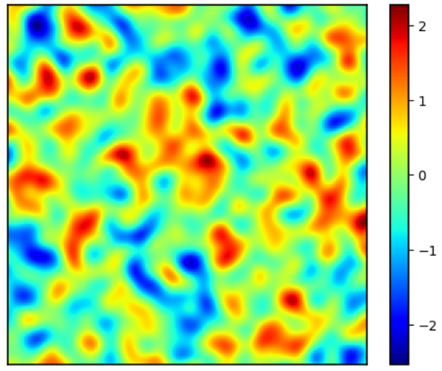
As a coefficient function in diffusion equation we use Gaussian random field (GRF) with efficient realization in parafields library[1] (Figure 2). The forcing term f is sampled from the standard normal distribution and each PDE is discretized using the 5-point finite difference method.

We generate four different datasets with different complexity for each grid value from {32, 64, 128}. Contrast in datasets is controlled with a variance in coefficient function GRF and takes value in {0.1, 0.5, 0.7}. Datasets are discretized with finite difference method with five-point stencil. One can find greater details about datasets in Appendix A.1

[1] https://github.com/parafields/parafield