This blog post delivers the fundamental principles behind object detection and it's algorithms with rigorous intuition.Prerequisites : Some basic knowledge in Deep Learning / Machine Learning / Mathematics .CONTENTS
1.) What is object detection ?
2.) Explanation of some of the terminologies involved in object detection.
3.) Walk-through to ANN,CNN
4.) Principles behind SSD and simple implementation in python.
5.) Case study involving ENA24 dataset(detecting wildlife animals).
What is object detection? It is a technique in computer vision, which is used to identify and locate objects in an image or video. The camera application deployed in recent computers uses object detection to identify face(s).There are many applications to it ranging from medical domain to more advanced domain like space research. There are many terminologies (jargon's) associated with object detection technology .We will discuss some of them in detail .
1.) Object : A material thing that can be seen and touched. In the computer vision community, it is considered as a group of pixels in an image or video which represent an material.In the above image, both apple and banana is an object. If you notice the image carefully, we can infer that a group of yellow colored pixels with a curvy structure forms an banana. Similarly, a group of red colored pixels with some structure forms an apple. So, basically most of the object detection algorithms involves in finding the common structure which forms an object.2.) Bounding box : It is an geometrical figure (square,circle,etc.,) which encloses the object of interest. If you look at the above image, the red colored rectangle depicts an bounding box. It encloses the apple(object) in the image.Similarly,the blue colored rectangle which encloses the banana(object) in the image depicts an bounding box. This bounding box is also called as ground-truth bounding box, as it is not generated by the object detection algorithm, rather it is already given .3.) Anchor box : It is an geometrical figure (square,circle,etc.,) which is generated by the object detection algorithm in order to identify and locate an object in an image. This definition will make more sense, when we try to discuss SSD.In the above image, the object of interest is the truck. The bounding box(ground-truth box) is the black colored rectangle. The goal of the algorithm is to predict the ground-truth box and the object contained in it.For that, it proposes multiple anchor boxes and filters out some of them based on certain criteria. Don't feel intimidated if you don't understand. We will discuss these ideas in more detail in the later part.4.) Category or class : This defines a name for an object . In the above image ,banana is the class(category) of the object enclosed in the blue colored rectangle. We can even call it as a fruit. Usually, we keep it simple.Artificial Neural Network(s).
1.) Linear neural network(s).
We will discuss this concept through an detailed example. Suppose you are at the market for buying some vegetable(s) .The price chart for the vegetable(s) is shown below .
You decided to buy three vegetables from the shop. But the price for three vegetables is not provided in the chart. It is our job to calculate the price and buy it. The price doesn't change , depending upon the quantity you purchase. What does it mean ? . Suppose, the price for single vegetable is P, then the price for five vegetable(s) is 5 (quantity) * P (price for single vegetable) . What does it convey ? If we find the price for a single vegetable, then we can easily find the price for arbitrary number of vegetables. How will you find ? Read this post , if you're truly hungry!!!
Let us use mathematics to solve our problem.
Let us denote the price for one vegetable as P Let us denote the quantity(total number of vegetables) as QTherefore, the price for Q number of items is P * QTherefore, our goal is to find P . If we find P , then we can easily calculate the price for any number of vegetables.
With the table given above , we can write the data in mathematical format as follows :
10 = P * 5 ; 12 = P * 6 ; 20 = P * 10 ; 44 = P * 22 . Our job is to find the P.
Let us assume , we have found the P . Then , we can conclude that :
(10 - P*5 ) + (12 - P*6) + (20 - P*10) + (44 - P*22) = 0 - (1)
We can also write the above equation as follows:
(10 - P*5)^2 + (12 - P*6)^2 + (20 - P*10)^2 + (44 - P*22)^2 = 0 -(2)
Both the equation are same, since both evaluates to zero . We call the above equation as loss or energy equation in the deep learning jargon. To call it as a function , we take the parameter as P . Therefore, the loss function is defined as :
L (P) = f( P ) , where f is another function. Here , in this example it is a sum of the squares of the differences between the true and the predicted value(s). Essentially , we need to find a P , such that L (P) = 0 . Since, we are finding a parameter such that it satisfies some constraint, it is called an optimization problem (with constraint). There are many methods to solve problems in optimization. One such method is called as gradient descent .
Gradient descent : 1.) Pose the objective or loss function .2.) Compute the derivative of the objective function with respect to the parameters of the function.3.) Displace the parameter in opposite to the gradient vector (generalization of derivative).It is a simple calculus exercise. You can try solve it on your own !!Why we call it as a network ?If we are trying to solve for multiple parameters, then it is termed as network of parameters hence the name linear neural network. The linear term arises , due to the fact that the function we are going to learn in the end is a linear function with respect to its inputs.
2.) Non-linear neural networks :
Suppose in the same example , if the relation looks like this :
Total price = e ^ (P*Q) . It is a non-linear function , since it's derivative term is not an constant !! Therefore , the function we are trying to approximate is an non-linear function . Hence, we coin the name as non-linear neural networks.
How do we solve this problem ?
If we try to approximate this function using an polynomial functions, then we need infinite amount of them to give a better approximation (Taylor series) . It is not possible to wait and compute infinite terms . What can we do about this ? . Well, we can try stacking simple non-linear functions (sigmoid function( crawl Wikipedia ) ) and then approximate our function. The sigmoid function has certain parameters involved in it. Use gradient descent and try optimizing the parameters with respect to the objective function.
That was a quick introduction to neural networks without much concentrating on its history and other stuff . Next , we move on to the discussion of convolutional neural networks .
Convolutional neural networks :
It's mostly an engineering hack, if we it look from the bottom . It exploits the core properties of the image . The core properties of the images are :
1.) Local features. 2.) Features are location independent ( It can be seen anywhere in the image ) .So to get better results on the problems involving images , the network must be designed in accordance with the above properties.
1.) Network must try to detect local features .2.) It must exploit translational invariance ( Even, if the features are displaced in the image the network must correctly identify it ).How is it designed ?
1.) To use the property numbered one , the network only considers a part of the input in a given time. This way , the network can identify local features in the input . Therefore , in a given layer we consider a subset of features from the superset of the overall features . This is usually implemented (not so) in practice by considering a weight matrix which has zeros in the place where the weights tries to focus outside the part of the input .2.) To use the property numbered two , the network must be designed in such a way that it slides across the input to find the possible locations where the feature(s) are present. The sliding window can be controlled by some parameter(s). One such way to implement this method is by defining a Toeplitz matrix (Refer Wikipedia to get more on this ) .Visual inspection :
Property 1:
Color code of the weight matrix : Black - zero White - non-zero quantity .
The zero in the weight vector nullifies the input at that location. Hence, it don't consider. Therefore , we exploited the property of locality .
Property 2 :
As you can see from the above gif , that the same weights are convolved with the image in different locations . Hence , we exploited the property of translational invariance .
There are many fundamental mathematical principles behind convolution and it's types . The discussion of that is beyond the scope of this post. Hence, we can safely skip that .
Principles behind SSD
It's an object detection algorithm which in a single-shot identifies and locates multiple objects in an image. We will discuss this algorithm with some examples . The subsequent material covered in this post will use these :
1.) MXNet deep learning framework. To install this framework, please feel free to surf the web for it's documentation.
2.) Python. To install this programming language, please feel free to surf the web for it's documentation.
3.) Some concepts in mathematics.( Linear Algebra, Vector calculus , Probability theory).
The best way to learn something is by starting from the foundations . We will use the same here . We will start by first building the Lego blocks and then we can finally construct our kingdom. We are going to consider an simple example to explain the details behind SSD. Later on this post, we will solve a complex problem.
Building blocks of SSD :
1.) Bounding boxLet's import some libraries import mxnet,d2l
from d2l import mxnet as d2l
from mxnet import np,npx
npx.set_np()Let's read an image image= mxnet.image.imread('H.jpg')
print("Number of channels ",image.shape[-1])
print("Image (height,width) ",image.shape[0],image.shape[1])
d2l.plt.imshow(image.asnumpy())Number of channels 3
Image (height , width) 200 200
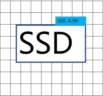
The above image is drawn using Microsoft White board. It is an picture with the letter 'H' in it. The job of any algorithm in the field of object detection is to identify the class or category of the object in the image and enclose it using an anchor box. Since, we are aware of the alphabets in the English language from our childhood we can easily spot it out. Therefore, we need to teach the model to do the same. We must manually label the above image by mentioning the bounding box of the letter 'H' and its category('H'). Once we have done this , we train the model to correctly identify it.
How to draw the bounding box? There are many tools available online and offline to do this task. One such tool is LabelImg. I used this tool to draw the bounding box around the object. Since we are dealing with one image ,we can itself do it. A bounding box is specified by four coordinates.( X_left , Y_left , X_right , Y_right ) . For the above image, the coordinates are: ( 45 , 32 , 150 , 170 ) . How I came up with this ? It's a small exercise left to the readers. Hint : The origin is the top left corner and the positive x-axis are right to it and the positive y-axis are downwards from the origin.
We will try to visualize this by writing some code
anchor_box_coordinates=[45,32,150,170]

def bbox_to_rect(bbox, color):
    """Convert bounding box to matplotlib format."""
    # Convert the bounding box (top-left x, top-left y, bottom-right x,
    # bottom-right y) format to matplotlib format: ((upper-left x,
    # upper-left y), width, height)
    return d2l.plt.Rectangle(
        xy=(bbox[0], bbox[1]), width=bbox[2]-bbox[0], height=bbox[3]-bbox[1],
        fill=False, edgecolor=color, linewidth=2)

fig = d2l.plt.imshow(img.asnumpy())
fig.axes.add_patch(bbox_to_rect(anchor_box_coordinates, 'blue'))
d2l.plt.show()
The bounding box is perfectly enclosing the object ('H').
2.) Convolutional neural network: We need some mechanism to identify and locate the letter 'H' in the image. We use convolutional neural network to perform this task. What does it do ?.We already mentioned in the beginning of this post, that an object is nothing but a collection of pixels with some structure. If we identify the structure and the group of pixels, we can easily spot the object in it. How do we do it ?.If we look carefully in the above image, the letter H contains two vertical edges and one horizontal edge. This is somewhat unique to this object. If we design an algorithm to find vertical and horizontal edges in an image , we can essentially detect the presence of the letter H. This is what exactly an convolutional neural network does. It inherits the principles of pattern matching and tries to use it to match features. We use what is called as a filter to accomplish this task.Filter to detect horizontal edges : How to design an filter , which detects the horizontal edges ? . We need to first understand the properties of the horizontal edges in order to design such filters .
1.) F( x , y + h ) - F(x , y ) / h turns out to be approximately zero . If we calculate the gradient by displacing in the x-direction then the quantity turns out to be very small .
2.) F( x + h , y ) - F ( x , y ) / h turns out to be a large quantity. At an edge , there will be an large difference in the vertical direction.
The variable h turns out to be 1 for an image. I leave it as a exercise to the readers as why is it so ? ...
The above mentioned equations has a special name called gradient
Let's code this up in python🎈kernel=np.array([[1,1,1],[0,0,0],[-1,-1,-1]])
kernel=np.expand_dims(kernel,axis=0)
kernel=np.concatenate([kernel,kernel,kernel],axis=0)
print(kernel,"\n")
print(kernel.shape)We don't need to code the convolution operation from scratch. The convolution operation is efficiently implemented in MXNet framework.
conv=mxnet.gluon.nn.Conv2D(3,3,padding=1,in_channels=3)
conv.initialize(init=mxnet.init.Constant(kernel))
print(conv.weight.data())
Let's perform the horizontal edge detection in our image.image=img.transpose(2,0,1)
image=np.expand_dims(image,axis=0)
image=image.astype('float32')
filtered=conv(image)
print(filtered)A larger magnitude of values represent an horizontal edge in the image. It is same as an classification problem. Assume we have two classes {0,1}, where 1 represents the presence of horizontal edge and 0 doesn't. We normally define our problem like this.
Find a w such that w.x >=c if x belongs to 1 and w.x < c if x belongs to 0 . Here x is nothing but the image and w is the kernel matrix. We need to figure out the c. It's a small exercise left out to the readers. Hint: Look into the values in the final matrix and figure out the value of c.
Similarly, the same set of procedure with different kernel matrix can be adopted to detect vertical edges. Please feel free to try and implement this. For this image , we could easily figure out the kernel matrix and perform the detection of the letter in the image. For some image involving many details, it is harder to find the suitable kernel matrix. Therefore, we need some mechanism which automate this process.
1.) Randomly initialize the values of w.
2) Perform the convolution operation with the image.
3) Define the loss function which takes w as the argument.
4) Backpropagate through the network to find the gradient of loss function with respect to the w vector.
5) Displace the w vector in the opposite direction of the gradient vector.
6) Perform 2 - 5 until convergence.
We will first implement the convolutional neural networkclass Convolution(mxnet.gluon.nn.Block):
def __init__(self):
super().__init__()
self.conv1 = mxnet.gluon.nn.Conv2D(channels=3,kernel_size=3,padding=1)
self.bn1 = mxnet.gluon.nn.BatchNorm()
self.conv2 = mxnet.gluon.nn.Conv2D(channels=3,kernel_size=3,padding=1)
self.bn2 = mxnet.gluon.nn.BatchNorm()
def forward(self,x):
x=npx.relu(self.bn1(self.conv1(x)))
x=npx.relu(self.bn2(self.conv2(x)))
return xconv = Convolution()
conv.initialize()
image=np.expand_dims(img,axis=0)
image=image.astype('float32')
print(conv(image))We initialized the values in the kernel matrix randomly. Then, we convolved the image with the kernel matrix.
3.) Anchor box generation :We solved the problem of recognizing the letter H in an image. Our next task is to identify the exact location of that letter H in the image. More precisely, we need to find the top left and bottom right coordinates of the rectangle (aka anchor box) which encloses the letter H. The problem here is slightly tricky. The letter H could be possibly anywhere in the image. We can't arguably guess a particular region in the image where the object(letter 'H') could be. There are some complex algorithms designed for such things. It has it's own pro's and con's. We will look into a naïve approach to solve this problem. What it could be ? . A simple solution is to generate all possible rectangles which is bounded by the image. How many such rectangles are possible ? A rectangle is defined by two coordinates namely ( X_left , Y_left , X_right , Y_right ). On a cartesian coordinate system, each value in the tuple has two degrees of freedom. Therefore, if the image's height and width are termed as h and w then there are totally s*s*s*s rectangles possible where s = max( h, w ). It's again a cute little exercise for the reader's to figure it out. In the algorithm paradigm, the cost of computing all possible rectangles is O ( n*n*n*n ) which is not feasible for practical purposes. We need to somewhat reduce this cost of operation. Not all the rectangles are useful. We can enclose a smaller rectangle with a larger one. What does it convey ? We don't need to possibly construct s*s*s*s rectangles. Some rectangles can be well approximated by others with small error. MXNet framework implements one such approach to solve this problem.
MXNet framework expects two things to construct anchor boxes.
1.) Size of the anchor box : It is a real number which belongs to the interval (0, 1]. This essentially tells how much proportion of the original image does the anchor box need to cover. If the size happens to be 1, then the anchor box covers the entire image.
2.) Ratio of the anchor box : It is a real number. It is also called as aspect ratio. It is defined as : r = width/ height . This ratio signifies the height and width of the anchor box. If r happens to be 2, then width is double the time height.
S = { s1, s2, . . . . sm } ; R = { r1, r2, r3,...... rn } where S:= set of sizes and R:= set of ratios for the anchor boxes. The number of anchor boxes generated would be m+n-1. The ordering is defined as follows :
( s1 , r1 ) , ( s1 , r2 ) ,…, ( s1 , rn ) , ( s2 , r1 ) , ( s3 , r1 ) ,…, ( sm , r1 ).
Let the image height be h and width be w. The image is typically visualized as a matrix with size (h , w ) where h is the number of rows and w is the number of columns. We generate ( m + n - 1 ) anchor boxes at each ( i , j )
position in the matrix as the center, where 0 <= i <= h and 0 <=j <=w . Therefore, total number of anchor boxes generated are w * h * ( m + n - 1 )
position in the matrix as the center, where 0 <= i <= h and 0 <=j <=w . Therefore, total number of anchor boxes generated are w * h * ( m + n - 1 )
We don't need to write an algorithm to generate the anchor boxes. It is already implemented in the MXNet framework. We will see how to utilize it.
We will first define a utility function to display the anchor boxes in the image.
#A simple routine to draw the rectangle specified by the coordinates.
#To have further details,please free to look into matplotlib documentation.
def bbox_plot(bbox,color):
    return d2l.plt.Rectangle(
        xy=(bbox[0], bbox[1]), width=bbox[2]-bbox[0], height=bbox[3]-bbox[1],
        fill=False, edgecolor=color, linewidth=2)

#This routine is to plot 'n' number of bounding boxes.
#All the code is implemented using matplotlib.
#We first draw the rectangle and define the patch to it by adding an text.

def multi_bbox(axes,bbox,labels,colors,size):
    for i,b in enumerate(bbox):
        if b[0]!=-size:
            c=colors[i]
            l=labels[i]
            rectangle=bbox_plot(b,c)
            axes.add_patch(rectangle)
            t_color='w'
            axes.text(rectangle.xy[0], rectangle.xy[1], l,
                          va='center', ha='center', fontsize=9, color=t_color,
                          bbox=dict(facecolor=c, lw=0))
We will define the sizes and the ratios for the anchor boxes.
sizes=[[0.27,0.44,0.52,0.62,0.71,0.85]]
ratios=[[1,1.5,2,2.2]]
#This code is taken from the matplotlib documentation.
#It is used to return the colors for the edges in the matplotlib library
prop_cycle = plt.rcParams['axes.prop_cycle']
colors = prop_cycle.by_key()['color']
image=mxnet.image.imread('/content/sample.PNG')
image=transforms.Resize(13)(image)
anchors=mxnet.npx.multibox_prior(image,sizes=sizes,ratios=ratios)
anchors=anchors.reshape(13,13,9,4)
anchors=anchors[5,5,:,:]
fig=d2l.plt.imshow(image.asnumpy())
scale=np.array([[13,13,13,13]]).as_in_context(device)
multi_bbox(fig.axes,a*scale,['' for i in anchors],colors[:9],13)We are visualizing all the anchors generated using (5,5) as the center.
4.) Category prediction :We have now the set of anchor boxes for an image. Not all anchor boxes encloses an object. Some of the anchor boxes doesn't even enclose an object of interest. This is where the crux of the SSD algorithm comes into play.
SSD algorithm :
1.) Propose a set of anchor boxes for an image.
2.) Label each anchor box with the category of the object which it encloses. If some anchor boxes doesn't enclose an object , label them as 'background'. How we label each anchor boxes ? Let's assume we have the ground truth bounding box for the letter 'H' . We generate ( n + m - 1 ) anchor boxes. Not all the anchor boxes encloses the letter 'H' . How do we measure this ? We define a term called IOU ( Intersection over Union ) .
G : = set of pixel values belonging to the ground truth anchor box
A : = set of pixel values belonging to the proposed anchor box
IOU :- |G ⨅ A | / | G U A |. If IOU is higher, then the bounding box and the anchor box are closer. So , basically we assign the category i to the anchor box j if IOU (bounding box m , anchor box j ) > 0.5 where i is the name of the category contained in the bounding box m.
3.) In the dataset , we have two pairs. The first item in the pair is the image and the second one is the bounding boxes of the object in that image. Next , compute the offsets of the anchor boxes from the original bounding box where there is a object contained in the anchor box. These offsets are defined as :
x_a and y_a are the center coordinates of the anchor box
x_b and y_b are the center coordinates of the bounding box
h_a and w_a are the height and width of the anchor box
h_b and w_b are the height and width of the bounding box
Why this weird formula to compute the offsets ? . Well , the reason is to have some normalized value such that it doesn't differ much if we choose some scaled version of the image. Don't get intimidated if you can't understand it. Just take it for granted.
4.) How to turn this into a supervised problem ? . We have the ground truth category for each anchor boxes and the offsets for each anchor boxes. We can use some network to output these values and we can define a loss function to penalize if it goes wrong. Then we can backpropagate through the network to adjust the parameters in order to reach a minimum loss.
Why does this needs to work ? Everybody can understand the steps, but not all can understand why it needs to work this way ? . To understand this, we need to first understand the concept of receptive field. When we are performing the convolution operation , we are basically looking at a local neighborhood of the input image. Each cell in the output matrix (matrix obtained by convolving the image with the kernel matrix ) has some correspondence with a local region in the image. As we go deep in the convolutional network, the receptive field increases ( it is a region in the input where the cell of the output matrix corresponds to ). So, if we make a classification layer at the very end of the network we are basically classifying objects with larger size. If we make a classification layer at the front of the network , we can classify objects with smaller size (since, it has a less receptive field ). Using this fact , we can design our algorithm to classify and detect objects of various kinds and sizes. Is it necessary to have a deep network to classify larger sized objects ? Not so.. We could have different sized kernel matrix at a layer and concatenate them to do the same thing. This is basically an inception network.
How to design a layer to output the predictions for the category contained in the anchor boxes ? We could use a linear layer to perform this operation. But the cost of operation is high, since it involves more parameters. It's again a small exercise to prove the former mentioned statement. An alternate solution is to use convolution layer to output the predictions. This has lesser parameters and also works better than a linear layer.
Let's code this up in python
def class_predictions(num_anchors , num_categories):
    return mxnet.gluon.nn.Conv2D( num_anchors * (num_categories + 1) , kernel_size=3,padding=1)
For each pixel in the image , we have generated (n + m - 1 ) anchor boxes already. For each anchor box , we need to label them with the category of the object it encloses. Therefore each pixel has ( n + m - 1 ) * (num_categories + 1 ) values , where n + m - 1 is the number of anchors. Pause for a minute and digest it.
Let's code the anchor boxes offset predictions layer.
def anchorbox_offsets(num_anchors):
    return nn.Conv2D(num_anchors * 4, kernel_size=3, padding=1)
We already discussed about the offset values of the anchor boxes in detail. For each anchor box, we have four offset values. Therefore there are total of 4 * num_anchors values for a given pixel.
We have everything to code up the SSD algorithm. We have looked at each segment in detail. Now , we are going to merge all these up and implement the SSD algorithm.
Let's do it !!!
import mxnet,d2l
from mxnet import np,npx
from mxnet.gluon import nn
npx.set_np()
We are just importing a set of libraries.
class Convolution(nn.Block):
      def __init__(self):
          super().__init__()
          self.conv1=nn.Conv2D(channels=3,kernel_size=3,padding=1,strides=2)
          self.bn1=nn.BatchNorm()
          self.conv2=nn.Conv2D(channels=3,kernel_size=3,padding=1,strides=2)
          self.bn2=nn.BatchNorm()
      def forward(self,x):
          x=npx.relu(self.bn1(self.conv1(x)))
          x=npx.relu(self.bn2(self.conv2(x)))
          return x
The size of the input image is : 200 , 200
We have two convolution blocks with strides as 2 for each one .
Therefore by using some simple math , we get the output shape as :
( 1 , 3 , 50 , 50 ) where 1 refers to the batch size.
def class_predictions(num_anchors,num_categories):
    return nn.Conv2D(num_anchors*(num_categories+1),kernel_size=3,padding=1)

def anchorbox_offsets(num_anchors):
    return nn.Conv2D(num_anchors*4,kernel_size=3,padding=1)
We already discussed about the above layers in detail.
class SSD(nn.Block):

      def __init__(self):

          super().__init__()
          self.sizes=[0.27,0.44,0.52,0.62,0.71,0.85]
          self.ratios=[1,1.5,2,2.2]
          self.num_anchors = len(self.sizes) + len(self.ratios) -1
          self.basenet=Convolution()
          self.class_predictions=class_predictions(self.num_anchors,1)
          self.anchorbox_offset=anchorbox_offsets(self.num_anchors)

      def forward(self,x):

          x=self.basenet(x)
          anchors=npx.multibox_prior(x,self.sizes,self.ratios)
          class_predictions= self.class_predictions(x)
          anchorbox_offsets= self.anchorbox_offset(x)

          anchors = anchors.reshape(-1,self.num_anchors*50*50,4)
          class_predictions = class_predictions.reshape(-1,self.num_anchors*50*50,2)
          anchorbox_offsets = anchorbox_offsets.reshape(-1,self.num_anchors*50*50*4)

          return anchors,class_predictions,anchorbox_offsets
ssd=SSD()
ssd.initialize()x=np.ones(shape=(1,3,200,200))
a,c,b=ssd(x)( 1 , 18 , 50 , 50 )
a.shape,c.shape,b.shape( (1 , 22500 , 4) , (1 , 22500 , 2) , (1 , 90000) )
1.) We passed our input image to the convolutional neural network to get the tensor with the features extracted from the image.
2.) We generated anchor boxes by using the size of the feature tensor.
3.) We get predictions for the ground truth category by passing into the category prediction layer.
4.) We get predictions for the ground truth offsets by passing into the offsets prediction layer.
5.) Finally we reshape the predictions to be compatible with the MXNet framework. It's not hard to find why this needs to be done.
The next step is to define the loss functions for our model. There are two loss functions to be defined.
1.) SoftMax Cross Entropy Loss :2.) L1Loss :category_loss = mxnet.gluon.loss.SoftmaxCrossEntropyLoss()
offset_loss= mxnet.gluon.loss.L1Loss()Now , we need to define the optimizer. The job of the optimizer is to update the trainable parameters of the model with some predefined rules. We are going to use Stochastic Gradient Descent with minibatch of size 1 and learning rate of 0.01 . Before declaring the optimizer , we need to initialize the model and pass in some input. This is for some optimization purpose .
model = SSD ()
model.initialize()
x = np.ones(shape=(1,3,200,200))
anchor,class_predictions,offsets = model(x)
trainer = mxnet.gluon.Trainer ( model.collect_params() , 'sgd' , {'learning_rate':0.01} )collect_params method returns the trainable parameters of the model which is passed.
Our next task is to define the procedure to train our model. We will define a simple routine for training our model. We will look more into it when we visit our case study.
def train(image,bounding_box,num_epochs):

    for epoch in range(num_epochs):
	with mxnet.autograd.record():
             anchors,class_predictions,offset_predictions = model(image)
             bbox_label,bbox_mask,class_truth = npx.multibox_target(anchors,bounding_box,class_predictions.transpose(0,2,1
             l=category_loss(class_predictions,class_truth) + offset_loss(offset_predictions*bbox_masks , bbox_labels*bbox_masks)
        l.backward()
        trainer.step(1)
multibox_target function is used to label the anchor boxes with the offset values and the category of the object it encloses.
autograd.record context is used to record the computation graph of our model for computing the intermediate gradients.
backward method is used to backpropagate through the network to actually compute the gradients with respect to the variable on which it is get invoked. Here, we are calculating the gradients with respect to the loss function.
The step method in the trainer object is used to displace the parameters in the opposite direction of the gradient.
We will see the output of the training routine and other details in our case study.
How do we do inference ?It's very easy to do the inference. We pass in our image to the model. We get the predictions for the classes contained in the object and the offset values. Using the SoftMax and argmax function , we get the highest probable category for each anchor box. We apply Non-max suppression algorithm on top of the anchor boxes. We filter out and produce the final output. The core idea of Non-max suppression algorithm is to eliminate the similar anchor boxes. For a prediction bounding box BB, the model calculates the predicted probability for each category. Assume the largest predicted probability is pp, the category corresponding to this probability is the predicted category of BB. We also refer to pp as the confidence level of prediction bounding box BB. On the same image, we sort the prediction bounding boxes with predicted categories other than background by confidence level from high to low, and obtain the list LL. Select the prediction bounding box B1B1 with highest confidence level from LL as a baseline and remove all non-benchmark prediction bounding boxes with an IOU with B1B1 greater than a certain threshold from LL. The threshold here is a preset hyperparameter. At this point, LL retains the prediction bounding box with the highest confidence level and removes other prediction bounding boxes similar to it. Next, select the prediction bounding box B2B2 with the second highest confidence level from LL as a baseline, and remove all non-benchmark prediction bounding boxes with an IOU with B2B2 greater than a certain threshold from LL. Repeat this process until all prediction bounding boxes in LL have been used as a baseline. At this time, the IOU of any pair of prediction bounding boxes in LL is less than the threshold. Finally, output all prediction bounding boxes in the list LL.
def inference(image):
    anchors, class_preds, offset_preds = model(image)
    class_probs = npx.softmax(class_preds).transpose(0, 2, 1)
    output = npx.multibox_detection(class_probs, offset_preds, anchors)
    idx = [i for i, row in enumerate(output[0]) if row[0] != -1]
    return output[0, idx]
multibox_detection function is used to perform Non-max suppression on the anchor boxes. It returns the filtered anchor boxes with the coordinates and the probability of the category given the anchor box. This probability value is used for thresholding logic. We can set the threshold to be in the range (0,1] and filter the anchor boxes. Depending upon the threshold value, the results may differ. It is left to the readers to implement this routine.
We came to the end of this section. We covered the details behind the SSD algorithm and some cup of intuition. Next , we will solve a real word problem with SSD algorithm.
Let's get started.Description
Real word problem
Problem Statement :1.) Given an wildlife image, identify and produce anchor boxes such that it covers the animals or any objects in the wildlife.
2.) This could be useful to monitor wildlife animals to safeguard them.
2.) This could be useful to monitor wildlife animals to safeguard them.
Useful Links :http://lila.science/datasets/ena24detection
https://awionline.org/content/what-you-can-do-wildlife
https://www.nature.com/scitable/knowledge/library/ethics-of-wildlife-management-and-conservation-what-80060473
https://www.nature.com/scitable/knowledge/library/ethics-of-wildlife-management-and-conservation-what-80060473
Business objectives and constraints :
1.) The images contained in the dataset contains many details, which is hard to model.
2.)The images provided in the dataset are taken from a single forest. Therefore, the idea of generalizability is a question.
3.) Micro F1 Score is vital, since all animals share many things as common. Therefore, we need to focus more on Micro F1 Score.
Installing the requirements :
#Installing the requirements.
!pip install mxnet-cu101==1.7.0
# !pip install tensorflow #Not required if you are in colaboratory notebook.
!pip install -U d2l
!pip install --upgrade mxnet-cu101 gluoncv
!pip install mxboard
# !pip install tensorboard #Not required if you are in colaboratory notebook
# !pip install tqdm #Not required if you are in colaboratory notebook
mxnet-cu101 framework comes with GPU enabled. If you want to have a version which only supports CPU , then remove -cu101 from the command.
gluoncv library is used in performing some transformations to the image.
mxboard library is used to visualize the model's output or some intermediate output in the tensorboard
Importing the required libraries :
#Importing the necessary modules.
import mxnet
from mxnet import np,npx,image
import os,json,tqdm
from tqdm import tqdm
os.environ['TF_CPP_MIN_LOG_LEVEL'] = '3'
from d2l import mxnet as d2l
import matplotlib.pyplot as plt
import time
from mxnet.gluon import nn
import gluoncv
from mxnet.gluon.data.vision import transforms
npx.set_np()
set_np function is to provide additional functionalities to the MXNet numpy array .
Downloading the dataset :
#wget command is used to download multiple files from the Internet.
!wget --header="Host: lilablobssc.blob.core.windows.net" --header="User-Agent: Mozilla/5.0 (X11; Linux x86_64) AppleWebKit/537.36 (KHTML, like Gecko) Chrome/84.0.4147.105 Safari/537.36" --header="Accept: text/html,application/xhtml+xml,application/xml;q=0.9,image/webp,image/apng,*/*;q=0.8,application/signed-exchange;v=b3;q=0.9" --header="Accept-Language: en-GB,en-US;q=0.9,en;q=0.8" --header="Referer: http://lila.science/datasets/ena24detection" "https://lilablobssc.blob.core.windows.net/ena24/ena24.zip" -c -O 'ena24.zip'
The above command is used to download the images from the server using wget command
#This command unzips the downloaded file
!unzip /content/ena24.zip -d /content/Images
We have extracted the downloaded files using the unzip command.
#wget command is used to download multiple files from the Internet.
!wget --header="Host: lilablobssc.blob.core.windows.net" --header="User-Agent: Mozilla/5.0 (X11; Linux x86_64) AppleWebKit/537.36 (KHTML, like Gecko) Chrome/84.0.4147.105 Safari/537.36" --header="Accept: text/html,application/xhtml+xml,application/xml;q=0.9,image/webp,image/apng,*/*;q=0.8,application/signed-exchange;v=b3;q=0.9" --header="Accept-Language: en-GB,en-US;q=0.9,en;q=0.8" --header="Referer: http://lila.science/datasets/ena24detection" "https://lilablobssc.blob.core.windows.net/ena24/ena24.json" -c -O 'ena24.json'
We are downloading the json file which contains some metadata about the dataset.
Exploratory Data Analysis:
Data preprocessing :#Using the json module,we are opening the json file
with open('ena24.json') as file:
info=json.load(file)We are loading the json file using load function.
#Displaying the keys contained in the json formatted file.
print(info.keys())
We are printing the keys contained in the json file.
#Displaying the content in the image key.
print(info['images'][:2])
We are printing the values stored in the images key.
#Displaying the content in the annotations key.
print(info['annotations'][0])
We are printing the values stored in the annotations key.
#Displaying the content in the categories key.
print(info['categories'][:2])
We are printing the values stored in the categories key.
#Displaying the content in the info key.
print(info['info'])
We are printing the values stored in the info key.
#Creating a empty dictionaries to store the details about images,annotations and categories.
images={}
annotations={}
categories={}
We are creating a set of dictionaries to store the information from the json file.
#We are extracting the information from the json file and storing it in separate dictionaries.
for i in info['images']:
    key=int(i['id'])
    images[key]={}
    images[key]['file_name']=i['file_name']
    images[key]['height']=i['height']
    images[key]['width']=i['width']
We are extracting the file name, height and width values from the images key and storing it in the dictionary.
#Displaying the information in the images dictionary.
images[8703]
#We are just appending the bounding boxes and category it belongs to.
#We are introducing a invariant called count.
#The count variable keeps track of the number of valid bouding boxes.
#More about the details regarding valid bounding boxes in the later part.
for i in info['annotations']:
key=int(i['image_id'])
if key not in annotations:
annotations[key]={}
annotations[key]['bbox']=[]
category=i['category_id']
i['bbox'].insert(0,category)
annotations[key]['bbox'].append(i['bbox'])
annotations[key]['count']=1
annotations[key]['category']=category
else:
category=i['category_id']
i['bbox'].insert(0,category)
annotations[key]['bbox'].append(i['bbox'])
annotations[key]['count']+=1We are extracting the bounding box coordinates and category values from the json file and storing it in our dictionary.
1.) The bounding box contains 4 values , ( X_left , Y_left, width , height)
2.) We append the category id in the bounding box list at the start for future purpose.
3.) Count is defined as the number of valid bounding boxes for an image.
4.) The meaning of valid makes sense, once we move further.
2.) We append the category id in the bounding box list at the start for future purpose.
3.) Count is defined as the number of valid bounding boxes for an image.
4.) The meaning of valid makes sense, once we move further.
#Displaying the keys in annotations.
annotations.keys()[:10]
#Displaying the values in the annotations dictionary
print(annotations.values()[0)#We are creating a map for storing the categories where key is the unique id and the value is the category it belongs to.
for i in info['categories']:
id=int(i['id'])
categories[id]=i['name']We are creating a dictionary to store the id and the name of the category.
#Displaying the category.
print(categories[10])
#We are using stochastic version of batch gradient descent.
#Therefore,it requires the data to be in batches.
#But the problem here is that,each image contains different number of bounding boxes.
#So,we find the image with maximum number of bouding boxes.
#We add extra illegal bounding boxes to other images until it reaches the maximum value.
#We add it with a special value ( -1 ).
#MxNet framework safely ignores the bounding boxes with -1 as labelled.
#We are also resizing the bounding box,since we are resizing the image to (200,200).
def bbox_transform(bbox,in_width,in_height,out_height,out_width,m,n):
temp=np.zeros(shape=(8,5))
temp[:m,1:]=gluoncv.data.transforms.bbox.resize(bbox[:,1:],(in_width,in_height),(out_width,out_height))
temp[:m,1:]/=200
temp[m:,:]=-1
temp[:m,0]=bbox[:m,0]
return temp#The format of the bounding box coordinates provided in the dataset are as follows:
# (x_min,y_min,width,height)
# We need to transform it into: (x_min,y_min,x_max,y_max)
# x_max= x_min + width
# y_max= y_min + height
# The above format is what MxNet expects.
# Also,MxNet is expecting the bounding box to be normalized i.e., it needs to be divided by the image's width and height.
def bbox_normalize(arg):
for i in arg.keys():
img_width,img_height=images[i]['width'],images[i]['height']
if type(annotations[i]['bbox'][0]) is list:
m=len(annotations[i]['bbox'])
for j in range(m):
v=annotations[i]['bbox'][j]
width=v[3]
height=v[4]
annotations[i]['bbox'][j][3]=annotations[i]['bbox'][j][1]+width
annotations[i]['bbox'][j][4]=annotations[i]['bbox'][j][2]+height
annotations[i]['bbox']=np.array(annotations[i]['bbox'])
annotations[i]['bbox']=bbox_transform(annotations[i]['bbox'],img_width,img_height,200,200,m,8)
else:
v=annotations[i]['bbox']
width=v[3]
height=v[4]
annotations[i]['bbox'][3]=annotations[i]['bbox'][1]+width
annotations[i]['bbox'][4]=annotations[i]['bbox'][2]+height
annotations[i]['bbox'][1]/=img_width
annotations[i]['bbox'][3]/=img_width
annotations[i]['bbox'][2]/=img_height
annotations[i]['bbox'][4]/=img_heightApplying some transformations to the bounding box
1.) We are using minibatch stochastic gradient descent for the optimization part.
1.) We are using minibatch stochastic gradient descent for the optimization part.
2.) It requires the data to be in batches. Therefore, the bounding boxes are expected to be in batches. The problem here is that different images have different bounding boxes. We can't process it in a single batch as it is varies in size.
3.)We find the maximum count of the bounding box and then pad all other bounding boxes with invalid bounding box for batch purpose.
4.) The bounding box coordinate's are given as (x_min,y_min,width,height).We need to transform it into (x_min,y_min,x_max,y_max), where x_max = x_min + width and y_max = y_min + height
bbox_normalize(annotations)Data Visualization:
#A simple routine to draw the rectangle specified by the coordinates.
#To have further details,please free to look into matplotlib documentation.
def bbox_plot(bbox,color):
    return d2l.plt.Rectangle(
        xy=(bbox[0], bbox[1]), width=bbox[2]-bbox[0], height=bbox[3]-bbox[1],
        fill=False, edgecolor=color, linewidth=2)
Rectangle function is used to draw the rectangle over an image if we specify the coordinates.
#This routine is to plot 'n' number of bounding boxes.
#All the code is implemented using matplotlib.
#We first draw the rectangle and define the patch to it by adding an text.

def multi_bbox(axes,bbox,labels,colors,size):
    for i,b in enumerate(bbox):
        if b[0]!=-size:
            c=colors[i]
            l=labels[i]
            rectangle=bbox_plot(b,c)
            axes.add_patch(rectangle)
            t_color='w'
            axes.text(rectangle.xy[0], rectangle.xy[1], l,
                          va='center', ha='center', fontsize=9, color=t_color,
                          bbox=dict(facecolor=c, lw=0))
Typically , an image contains multiple objects in it . Hence, there would be multiple bounding boxes in it. To draw multiple bounding boxes on an image , we just add the patch multiple times. To render a text on the edge of the rectangle , we use text method in the axes object.
#Displaying the sample bounding box.
#The value -1 in the array indicates that, it is a illegal bounding box present for creating a batch.
bbox=annotations[3]['bbox']
bbox
-1 indicates the presence of invalid bounding box. Different images have different number of bounding boxes. Since we train our model with a batch of data , we need everything to be in batches. We find the maximum number of bounding boxes an image can have and pad others with -1 till it reaches the maximum value. The range of values the bounding box takes is [0,1], since we divided by the width and height.
#We are reading the image using OpenCV
#We are resizing the image using Resize block (MxNet block)
#We are displaying the image with bounding boxes on it.
image=mxnet.image.imread('/content/ena24/3.jpg')
image=transforms.Resize(200)(image)
fig=d2l.plt.imshow(image.asnumpy())
multi_bbox(fig.axes,bbox[:,1:]*np.array([[200,200,200,200]]),[categories[int(i[0])] if int(i[0])!=-1 else 'Null' for i in bbox],['r' for i in range(9)],200)
#We are defining a count variable and storing the number of valid bounding boxes for each image.
counts=[]
for i in annotations.values():
counts.append(i['count'])The above routine appends the number of valid bounding boxes for an image in a list variable.
#This is just a simple plot describing the number of bounding boxes for each image.
#This plot shows that, the maximum number of bounding boxes for an single image is 8.
#Most of the images contains 4 or less number of bounding boxes.
d2l.plt.title('Bounding box id vs Number of bounding boxes')
d2l.plt.xlabel('Bounding box id')
d2l.plt.ylabel('Number of bounding box')
d2l.plt.plot(counts)
d2l.plt.show()
We plotted the number of bounding boxes for each image in our dataset.
#It calculates the maximum number of bounding box for an single image.
print(max(counts))
8
The maximum number of bounding box for an image in the entire dataset is 8.
#This simple routine calculates the area of the bounding boxes.
#It is to describe the sizes of the objects contained in the image.
#The formula is :
# (width * height)
# width= (x_max-x_min) and height= (y_max-y_min)
#The area values are bounded between [0,1], since we normalized them.

def calculate_area(bbox_dict):
    areas=[]
    for i in bbox_dict.keys():
        b=bbox_dict[i]['bbox']
        c=bbox_dict[i]['count']
        for j in range(c):
            temp=b[j]
            area=(temp[3]-temp[1])*(temp[4]-temp[2])
            areas.append(area.item())
    return areas

areas=calculate_area(annotations)
d2l.plt.ylabel('Area')
d2l.plt.xlabel('Bounding box')
d2l.plt.title('Area vs Bounding box id')
d2l.plt.plot(areas)
d2l.plt.show()
We plotted the are of the bounding boxes for each image. This value signifies the sizes of the objects in the image. It is very useful to know this information. If the sizes of the object are less than 0.2 (normalized value) , then identifying an object is quite hard. The values of the area are in the range (0,1] since we normalized the coordinates of the bounding boxes. We used the fact that : Area of a rectangle = Width * Height .
We will look more in the data visualization part , when we discuss about our final model.
Preparing the dataset.
1.) There are some images which are missing in the downloaded files which are mentioned in the json file .
2.) We will consider only the provided images.
#It uses the os module to store the list of files in the main variable.
main=os.listdir('/content/ena24')
main variable stores the list of names of the images.
#We are ignoring the '.jpg' expression for reading purpose.
main=[int(i[:-4]) for i in main]
The image names also includes the suffix '.jpg'. This routine is used to eliminate the suffix '.jpg'.
#Displaying the length of the dataset.
print(len(main))
8789
This routine is used to print the total length of the dataset ( total number of images with bounding boxes ) .
For training purpose, we need to split our dataset into train / test . We can split it randomly or using any other valid method since there is no time axis.
#Since, there is no notion of time axis, we can safely split the dataset randomly or using any valid method.
train_indices=main[:7031]
test_indices=main[7031:]
We are just splitting our dataset in the ratio 0.8 : 0.2 .
# TWe are inheriting from the Dataset abstract class.
# We are storing the indices,images and their responding annotations.
# We are storing the location where the dataset is stored in the local disk.
# The length method returns the number of valid examples for training the model.
# The getitem method is used to select an example from the list of examples and applies some transformations if it has.
class Ena24TrainDataset(mxnet.gluon.data.Dataset):

      def __init__(self,train_indices,images,annotations,root):

          super().__init__()
          self.train_indices=train_indices
          self.images=images
          self.annotations=annotations
          self.root=root

      def __len__(self):

          return len(self.train_indices)

      def __getitem__(self,idx):

          index=self.train_indices[idx]
          image=mxnet.image.imread(os.path.join(self.root,self.images[index]['file_name']))
          bbox=self.annotations[index]['bbox']

          return image,bbox
We created an class to define our data preparation process.
This class inherits from the Dataset class ( provided in the MXNet framework).
init method :len method :getitem method :We do the same for our test dataset.
# TWe are inheriting from the Dataset abstract class.
# We are storing the indices,images and their responding annotations.
# We are storing the location where the dataset is stored in the local disk.
# The length method returns the number of valid examples for training the model.
# The getitem method is used to select an example from the list of examples and applies some transformations if it has.
class Ena24TestDataset(mxnet.gluon.data.Dataset):

      def __init__(self,test_indices,images,annotations,root):

          super().__init__()
          self.test_indices=train_indices
          self.images=images
          self.annotations=annotations
          self.root=root

      def __len__(self):

          return len(self.test_indices)

      def __getitem__(self,idx):

          index=self.test_indices[idx]
          image=mxnet.image.imread(os.path.join(self.root,self.images[index]['file_name']))
          bbox=self.annotations[index]['bbox']

          return image,bbox
# We are setting the device variable to be the gpu context.
# This is done,so that we can load our data in the gpu.
device=mxnet.gpu(0)
We will train our model using the GPU. We define a variable called device which basically holds the logic for that.
# This function defines the transformation to the samples in the dataset.
# It resizes the image to be of (200,200) and normalizes them.
def custom_transformations(*sample):
    mean= np.array([0.485, 0.456, 0.406]).reshape(3,1,1)
    std=np.array([0.229, 0.224, 0.225]).reshape(3,1,1)
    img=sample[0]
    bbox=sample[1]
    img=transforms.Resize(200)(img)
    img=transforms.ToTensor()(img)
    img[:]-=mean
    img[:]/=std
    return (img.as_np_ndarray().as_in_context(device),bbox.as_in_context(device))
1. ) We normalize the image by ImageNet statistics .2. ) We resize the image to ( 200 , 200 ) .3. ) We convert into a ndarray Tensor ( it moves the channel dimension after the batch axis ) .4. ) We put the data in the GPU memory .#Creating a dataset object from the class we defined earlier.
train_data=Ena24TrainDataset(train_indices,images,annotations,'/content/ena24')We apply the above mentioned transformation to our dataset and create an dataset object out of it. This object encapsulates all the information required to create a data loader out of it .
#We are creating a dataloader object which encompasses the dataset object and is used to produce batches while training.
#We set the value of the shuffle parameter as True.This is done to change the order of dataset in each epoch.
#We declared the batch_size as 8.
train_dataloader=mxnet.gluon.data.DataLoader(train_data.transform(custom_transformations),batch_size=8,shuffle=True,last_batch='discard')
We create a data loader object from the dataset object .
1.) Batch size = 8
2.) We are shuffling the dataset , since we are going to iterate over the entire dataset multiple times. Bonus : Think about Stochastic Gradient Descent.
3.) We discard the last batch , since we need to perform some additional configuration to process that single one. It is unnecessary. Therefore , we can safely discard the last batch. Ambitious programmers can implement that routine if needed.
We will do the same for our test dataset.
#Creating a dataset object from the class we defined earlier.
test_data=Ena24TestDataset(test_indices,images,annotations,'/content/ena24')
#We are creating a dataloader object which encompasses the dataset object and is used to produce batches while training.
#We set the value of the shuffle parameter as True.This is done to change the order of dataset in each epoch.
#We declared the batch_size as 8.
test_dataloader=mxnet.gluon.data.DataLoader(test_data.transform(custom_transformations),batch_size=8,shuffle=True,last_batch='discard')We will create our base model which is a convolutional neural network. It is used to extract a latent representation of our input image by obeying the property of translational invariance and local features.
#This model is inspired from Inception network.
#We didn't use maxpooling layer.There is no reason behind it.It worked well without it.I heard Mr.Geoffrey Hinton saying that maxpooling layers are not good.
#All other traditional things are followed here.
class CustomConv(nn.HybridBlock):

      def __init__(self):
          super().__init__()
          self.conv31=nn.Conv2D(200,3,padding=1)
          self.conv51=nn.Conv2D(100,5,padding=2)
          self.conv71=nn.Conv2D(50,7,padding=3)
          self.conv11=nn.Conv2D(300,1)
          self.conv32=nn.Conv2D(350,3,padding=1,strides=2)
          self.conv33=nn.Conv2D(400,3,padding=1,strides=2)
          self.conv34=nn.Conv2D(450,3,padding=1,strides=2)
          self.conv35=nn.Conv2D(500,3,padding=1,strides=2)
          self.bn1=nn.BatchNorm()
          self.bn2=nn.BatchNorm()
          self.bn3=nn.BatchNorm()
          self.bn4=nn.BatchNorm()
          self.bn5=nn.BatchNorm()
          self.bn6=nn.BatchNorm()
          self.bn7=nn.BatchNorm()
          self.bn8=nn.BatchNorm()

      def hybrid_forward(self,F,x):

          y=F.npx.relu(self.bn1(self.conv31(x)))
          z=F.npx.relu(self.bn2(self.conv51(x)))
          t=F.npx.relu(self.bn3(self.conv71(x)))
          x=F.np.concatenate((y,z,t),axis=1)
          x=F.npx.relu(self.bn4(self.conv11(x)))
          x=F.npx.relu(self.bn5(self.conv32(x)))
          x=F.npx.relu(self.bn6(self.conv33(x)))
          x=F.npx.relu(self.bn7(self.conv34(x)))
          x=F.npx.relu(self.bn8(self.conv35(x)))
          return x
1.) This model inherits some of the properties from Inception network.
2.) The dataset contains objects in the images of varying sizes.
3.) To model this aspect of this dataset, we need to design our model in accordance with that .
4.) So, we used different size kernels at the first layer and appended it's activations at the feature dimension , so that it models the varying size property .
5.)The research paper containing SSD says to use multiple feature blocks and concatenate the activations, so that we can identify objects at varying sizes .
6.) The idea for using multiple feature blocks also helps in sampling the anchor boxes according to the size of the feature map . For eg , we can sample less number of anchor boxes for identifying large objects and more anchor boxes to identify small objects.
7.)In our approach , we sampled a fixed number of bounding boxes . To compensate it ,we introduced weighted loss .
8.) Rather than using multiple feature blocks, we used single feature block with different kernels . This is equivalent to the method discussed in the paper .
9.) Other than that, we used Relu , Batch Norm by following the traditional approach .
#Instantiating the class to create an object.
model=CustomConv()
We are creating an object named model from the class.
#Initializing the object.It is done for optimization part.To get more details about it,please free to look the MxNet documentation
model.initialize()
It initializes the trainable/non-trainable parameters in the model.
#Creating a sample input.
x=np.ones(shape=(1,3,200,200))
We define a sample input.
#Transforming the input by the rules specified by the model.
#Bonus: It is equivalent to calling model.forward(x) (A special __call __ method)
print(model(x).shape)
We transformed our sample input by the model definition.
#Routine to calculate the number of trainable parameters.
#It uses the method collect_params(), which inturn returns the parameters stored in the model's kvstore.
ans=0
for i in list(model.collect_params().values()):
    ans+=(i.data().size)
The above code snippet traverses the model's parameters and calculates the total size.
#Displaying the total parameters.
print("Total number of parameters ",ans)
Visualizing the model We need to first hybridize our model.
#The hybridize method is used to convert the model's definition to symbolic representation(Used in C++ inference).It is a advanced concept.
model.hybridize()
model(x).shape
We are just converting our model's computation graph to a symbolic representation.
#We are using the Mxboard library which internally integrates with tensorboard.
#We are using the SummaryWriter and defining a context to add the model to visualize it.
from mxboard import SummaryWriter
with SummaryWriter(logdir='./ena24_tensorboard/model1') as sw:
     sw.add_graph(model)
We have used SummaryWriter class from the mxboard library to log the computation graph of our model to the format required by the tensorboard.
add_graph method is used to convert the model's symbolic representation to the format required by the tensorboard.
#Magic command to use the tensorboard in the jupyter notebook.
%load_ext tensorboard
The above magic command is used to load the tensorboard in the jupyter notebook itself.
#Loading the tensorboard.
%tensorboard --logdir ./ena24_tensorboard/model1/
We normally invoke the tensorboard by specifying the directory location where the event files are residing.
This is how the computation graph looks like. PS : Sorry for the poor quality😐
Finally , we need to create a class which encapsulates all the information required to train our model.
#We are creating the final class to define all the methods and invariants for our final model.
#We define the sizes and ratios for the anchor boxes we are going to propose.
#We are defining a class prediction layer, which is a convolution block that transforms the input(batch_size,number of channels,height,width) to (batch_size,(number_of_anchors)*(num_classes+1),width,height)
#We are defining a bounding box prediciton layer,which is a convolution block that transforms the input(batch_size,number of channels,height,width) to (batch_size,(number_of_anchors)*4,width,height)
#We used convolution block,since it holds less number of parameters than a dense layer or any such.
#We are not using multi-stage blocks, so there is no need for concatenating the predictions at multiple stages.
#But still I implemented the routine for multi-stage blocks,for future purpose.

class Ena24SSD(nn.HybridBlock):

      def __init__(self):
          super(Ena24SSD,self).__init__()
          self.sizes=[[0.27,0.44,0.52,0.62,0.71,0.85]]
          self.ratios=[[1,1.5,2,2.2]]
          self.num_anchors=len(self.sizes[0])+len(self.ratios[0])-1
          self.num_classes=23
          self.class_predict=self.class_predictor()
          self.bbox_predict=self.bbox_predictor()
          self.features=CustomConv()

      def class_predictor(self):
          s=nn.HybridSequential()
          g=[nn.Conv2D(self.num_anchors*(self.num_classes+1),3,padding=1),nn.BatchNorm(),nn.Activation('softrelu')]
          s.add(*g)
          return s

      def bbox_predictor(self):
          b=nn.HybridSequential()
          f=[nn.Conv2D(kernel_size=3,padding=1,channels=380),nn.BatchNorm(),nn.Activation('relu')]
          s=[nn.Conv2D(kernel_size=3,padding=1,channels=220),nn.BatchNorm(),nn.Activation('relu')]
          t=[nn.Conv2D(kernel_size=3,padding=1,channels=120),nn.BatchNorm(),nn.Activation('relu')]
          fo=[nn.Conv2D(kernel_size=3,padding=1,channels=4*self.num_anchors),nn.BatchNorm(),nn.Activation('relu')]
          b.add(*f,*s,*t,*fo)
          return b

      def hybrid_forward(self, F, x, *args, **kwargs):
          feature=[]
          feature.append(self.features(x))

          cls_preds=F.npx.batch_flatten(F.np.transpose(self.class_predict(feature[0]),(0,2,3,1)))
          bbox_preds=F.npx.batch_flatten(F.np.transpose(self.bbox_predict(feature[0]),(0,2,3,1)))
          anchors=F.np.reshape(F.npx.multibox_prior(feature[0],self.sizes[0],self.ratios[0]),(1,-1))
          cls_preds=F.npx.reshape(cls_preds,(-2,-1,self.num_classes+1))
          bbox_preds=F.npx.reshape(bbox_preds,(-2,-1))
          anchors=F.np.reshape(anchors,(1,-1,4))
          return anchors,cls_preds,bbox_preds
We defined a class named Ena24SSD , which serves as the main class.
This class holds the definition for the anchor box offset predictions layer and class predictions layer.
It holds the definition for the base model also.
We define the anchor box sizes and their ratios in the class.
In the forward method , this model computes the predictions for the anchor box offsets and the predictions for the category from the feature map generated by the base model.
It concatenates all the predictions, so that it can be processed in batches.
#We are instantiating the class and creating an object.
model=Ena24SSD()
We are creating an object of this class.
#We are initializing the model.
model.initialize(ctx=device)
We are initializing and storing the model parameters in the GPU memory. The device variable basically holds the logic for it.
#We are transforming the image to anchors,class_predictions,boundingbox_offsets.
image=np.ones(shape=(1,3,200,200)).as_in_context(device)
anchors,class_predictions,boundingbox_predictions=model(image)
We created a dummy input in place of the image.
The input is transformed by the model into anchors , class_predictions , boundingbox_predictions.
#We are displaying the shape of the outputs returned by the model.
anchors.shape,class_predictions.shape,boundingbox_predictions.shape
#This code is taken from the matplotlib documentation.
#It is used to return the colors for the edges in the matplotlib library
prop_cycle = plt.rcParams['axes.prop_cycle']
colors = prop_cycle.by_key()['color']#Displaying the available colors.
print(colors)It is a list of available colors.
#We are visualizing the anchors on a dummy image.
#The anchor boxes are designed to cover all sizes of the object in an image.
#We used the multi_bbox function which was defined earlier in the notebook.
a=anchors.reshape(13,13,9,4)
a=a[5,5,:,:]

image=mxnet.image.imread('/content/sample.PNG')
image=transforms.Resize(13)(image)
fig=d2l.plt.imshow(image.asnumpy())
scale=np.array([[13,13,13,13]]).as_in_context(device)
multi_bbox(fig.axes,a*scale,['' for i in a],colors[:9],13)
We have reshaped our anchor array to (13 , 13 ,9 ,4) (13 , 13 ) -> ( w , h ).
We slice the array at ( 5 , 5 ) . It basically holds all the anchor box coordinates which are generated using ( 5 , 5 ) as their center.
We read an image for visualization purpose.
We resize the image to ( 13 , 13 ).
Since the coordinates of the anchor boxes are normalized , we need to scale it.
We visualize the anchor boxes over the image using multi_bbox function which we defined earlier.
#We are using the collect_params() method to display the parameters which the model holds.
print(model.collect_params())
Due to space constraint , the output is trimmed.
collect_params method returns the list of parameters object , which are stored in the dictionary.
#We are hybridizing the model.
model.hybridize()
a,c,b,=model(x.as_in_context(device))
We hybridized the model for visualizing it.
#We are exporting the model to tensorboard format.
from mxboard import SummaryWriter
with SummaryWriter(logdir='./ena24_tensorboard/model2') as sw:
     sw.add_graph(model)
We have already discussed about this snippet earlier.
#We are loading the tensorboard.
%tensorboard --logdir ./ena24_tensorboard/model2/
It looks messy 🙄
Metrics
#Micro F1 score is used to treat multiclass detection problem.We need to implement on our own(Not inplemented in the library itself).

class MicroF1Score(mxnet.gluon.nn.HybridBlock):

    def __init__(self,num_classes):
        super().__init__()
        self.classes=list(range(num_classes+1))
        self.true_pos=[0]*(len(self.classes)+1)
        self.false_pos=[0]*(len(self.classes)+1)
        self.false_neg=[0]*(len(self.classes)+1)

    def hybrid_forward(self,F,x):
        pred=x[0]
        true=x[1]

        for i in range(1,len(self.classes)):
            p=mxnet.np.equal(pred,i)
            t=mxnet.np.equal(true,i)
            true_positive=float((p*t).sum())
            false_positive=float(((true!=i)*p).sum())
            false_negative=float((t*(pred!=i)).sum())
            self.true_pos[i]=true_positive
            self.false_pos[i]=false_positive
            self.false_neg[i]=false_negative
        true_pos=sum(self.true_pos)
        false_pos=sum(self.false_pos)
        false_neg=sum(self.false_neg)
        if (true_pos+false_pos)==0:
            precision=0
        else:
            precision=true_pos/(true_pos+false_pos)
        if (true_pos+false_neg)==0:
            recall=0
        else:
            recall=true_pos/(true_pos+false_neg)
        if (precision+recall)==0:
            f1score=0
        else:
            f1score=(2*(precision*recall))/(precision+recall)
        return float(format(f1score,'.2g'))
There is no implementation for the Micro_F1 score in the MXNet framework. We need to implement our own routine for it.
The crux of the Micro_F1 metric is averaging the precision and recall across the different classes. This metric truly evaluates it. We used harmonic mean in place of the naïve average
#Overall accuracy
def evaluateclass(class_preds,class_labels):
    predictions=npx.softmax(class_preds).argmax(axis=-1)
    return ((predictions.astype(class_labels)==class_labels).mean()).item()
We are also interested in the accuracy. It calculates the number of matches between true and the predicted observations. It also normalizes it.
#Mean absolute deviation (for bounding box).
def evaluatebbox(bbox_preds,bbox_labels,bbox_masks):
    return ((np.abs((bbox_labels-bbox_preds)*bbox_masks)).mean()).item()
The above routine calculates the average deviations of the predicted anchor boxes offsets from the ground truth one.
Loss Function
#Since,it is a multiclass detection problem
classs_loss=mxnet.gluon.loss.SoftmaxCrossEntropyLoss()
#For boundning box offset loss
bbox_loss=mxnet.gluon.loss.L1Loss()

#Container for loss computation.
class LossBox:
    def __init__(self):
        self.weight=(np.ones(shape=(batch_size,num_anchors))).as_in_context(device)
        self.weight1=((np.ones(shape=(batch_size,num_anchors*4)))*2).as_in_context(device)
    def calculate_loss(self,class_preds,class_labels,bbox_preds,bbox_labels,bbox_masks,train):
        if train==1:
            weights=((self.weight*(class_labels!=0))*900)+((np.ones(shape=class_labels.shape,ctx=device))*100)
            loss_class=classs_loss(class_preds,class_labels,np.expand_dims(weights,axis=-1))
            loss_bbox=bbox_loss(bbox_preds*bbox_masks,bbox_labels*bbox_masks,self.weight1*bbox_masks)
        else:
            loss_class=classs_loss(class_preds,class_labels)
            loss_bbox=bbox_loss(bbox_preds*bbox_masks,bbox_labels*bbox_masks)
        return loss_bbox+loss_class
SoftmaxCrossEntropyLoss is used in classification settings.
L1Loss is used to define a measure for the deviations of the predicted observations from the true observations when the observations are real and used in regression settings.
The maximum number of objects contained in a single image is 8 in our case. Therefore, most of the anchor boxes have label as background. This badly affects the Micro_F1 score. To overcome it, we add weights to the observations where the anchor boxes are not labelled as background.
Optimization
#We are defining the trainer object.
#We are using Stochastic gradient descent in batches.
#We can use Adam,NaG,etc.
#The problem is,it itself contains some parameters.
#The sgd is working very well.
trainer=mxnet.gluon.Trainer(model.collect_params(),'sgd',{'learning_rate':0.01})
We used stochastic gradient descent optimizer with a learning rate of 0.01.
Training
#We are declaring some empty lists to store the metrics and losses.
train_loss_l=[]
test_loss_l=[]
train_f1_l=[]
test_f1_l=[]
train_accuracy_l=[]
test_accuracy_l=[]
train_mae_l=[]
test_mae_l=[]
num_epochs=50
We are declaring some empty lists to store the metrics and losses.
with SummaryWriter(logdir='./models/plots') as sw:

      for epoch in tqdm(range(num_epochs)):

          start=time.time()

          loss=0
          train_loss=0
          test_loss=0
          train_f1=0
          test_f1=0
          train_accuracy=0
          test_accuracy=0
          train_mae=0
          test_mae=0

          for data in train_dataloader:
              image,label=data[0],data[1]
              with mxnet.autograd.record():
                  anchors,class_predictions,bbox_predictions=model(image)
                  bbox_labels,bbox_masks,class_labels=npx.multibox_target(anchors,label,class_predictions.transpose(0,2,1))
                  l=(losses.calculate_loss(class_predictions,class_labels,bbox_predictions,bbox_labels,bbox_masks,1)).sum()
              loss=loss+(l.mean().item())
              l.backward()

              if len(train_loss_l)>=2:
                 if train_loss_l[-1]>=train_loss_l[-2]:
                    trainer.set_learning_rate(trainer.optimizer.lr/5)

              trainer.step(batch_size)

          train_loss=loss
          train_mae=evaluatebbox(bbox_predictions,bbox_labels,bbox_masks)
          class_p=(npx.softmax(class_predictions).argmax(axis=-1)).reshape(-1)
          class_l=class_labels.reshape(-1)
          train_f1=f1((class_p,class_l))
          train_accuracy=evaluateclass(class_predictions,class_labels)

          train_loss_l.append(train_loss)
          train_f1_l.append(train_f1)
          train_accuracy_l.append(train_accuracy)
          train_mae_l.appen
          test_f1_l.append(test_f1)d(train_mae)

          for data in test_dataloader:
              anchors,class_predictions,bbox_predictions=model(image)
              bbox_labels,bbox_masks,class_labels=npx.multibox_target(anchors,label,class_predictions.transpose(0,2,1))
              l=(losses.calculate_loss(class_predictions,class_labels,bbox_predictions,bbox_labels,bbox_masks,0)).sum()
              loss=loss+(l.mean().item())

          test_loss=loss
          test_mae=evaluatebbox(bbox_predictions,bbox_labels,bbox_masks)
          class_p=(npx.softmax(class_predictions).argmax(axis=-1)).reshape(-1)
          class_l=class_labels.reshape(-1)
          test_f1=f1((class_p,class_l))
          test_accuracy=evaluateclass(class_predictions,class_labels)

          test_loss_l.append(test_loss)
          test_accuracy_l.append(test_accuracy)
          test_mae_l.append(test_mae)


          sw.add_scalar(tag='Log_loss',value={'train':train_loss,'test':test_loss},global_step=epoch)
          sw.add_scalar(tag='Accuracy',value={'train':train_accuracy,'test':test_accuracy},global_step=epoch)
          sw.add_scalar(tag='MAe',value={'train':train_mae,'test':test_mae},global_step=epoch)
          sw.add_scalar(tag='Micro_F1',value={'train':train_f1,'test':test_f1},global_step=epoch)

          if train_f1>=0.8 and test_f1>=0.8:
             model.save_parameters('model_'+str(epoch))


          dicts=dict(model.collect_params())
          for i in dicts.keys():
              if i[-6:]=='weight':
                 sw.add_histogram(tag=i,values=dicts[i].data(),global_step=epoch,bins=200)
              else:
                  if i[-4:]=='bias':
                     sw.add_histogram(tag=i,values=dicts[i].data(),global_step=epoch)


          end=time.time()
          print("Time taken to run epoch ",epoch," ",(end-start)/60," minutes")
The above code segment defines the statements required for training the model.
As usual , we calculate the losses and backpropagate through the network to tune the learnable parameters.
We plot the loss , Micro_F1 , accuracy and mean absolute deviations of the offsets.
We used tensorboard for logging the distribution of weights , losses and metrics.
In the SummaryWriter context,we log various plots,histograms of our training process.
We normally transform the inputs given by the dataloader in batches by our model.
We used categorical cross entropy loss for the class probability
We used L1Loss for the anchor box offsets.
Once we calculate the loss,we backpropagate through the network and compute the intermediate gradients.
Then,by SGD we update the model's trainable parameters.
We do this for the entire dataset 50 times.
After everything is over, we visualize the entire training process via tensorboard(which we logged while training.)
#We are loading the tensorboard.
%tensorboard --logdir models/plots/
Color coding :Log loss :Accuracy :MAE (Mean absolute deviation ):Micro_F1 score :from prettytable import PrettyTable
table = PrettyTable()
table.field_names = [ 'Accuracy/train','Accuracy/test','Log_loss/train','Log_loss/test','MAe/train','MAe/test','Micro_F1/train','Micro_F1/test']
table.add_row([0.9988,0.9985,1.39,1.40,0.0025,0.0024,0.89,0.88])
print(table)We created a table using prettytable library to summarize our final observations in a tabular format .
model.save_parameters('model')save_parameters method is used to save the parameters of the model.
Inference :
#We are transforming the image
def image_transform(image):
    mean= np.array([0.485, 0.456, 0.406]).reshape(3,1,1)
    std=np.array([0.229, 0.224, 0.225]).reshape(3,1,1)
    image=transforms.ToTensor()(image)
    image[:]-=mean
    image[:]/=std
    return np.expand_dims((image.as_np_ndarray()),axis=0).as_in_context(device)


#Used to display the anchor boxes on the image.
def bbox_show(bbox,image):
    fig=d2l.plt.imshow(image)
    multi_bbox(fig.axes,bbox[:,1:]*np.array([[200,200,200,200]]),[categories[int(i[0])] if int(i[0])!=-1 else 'Null' for i in bbox],['r']*(bbox.shape[0]),200)


#This routine takes in the image location and applies the transformation specified by the model.
#It used non-max suppression to filter out the anchor boxes.
#It outputs the anchor boxes,if the class probability is higher than the threshold.

def prediction(image_location,threshold):
    image=mxnet.image.imread(image_location)
    image=transforms.Resize(200)(image)
    image_numpy=image.asnumpy()
    image=image_transform(image)
    anchors,class_predictions,bbox_offsets=model(image)
    class_predictions=npx.softmax(class_predictions)
    output=npx.multibox_detection(class_predictions.transpose(0,2,1),bbox_offsets,anchors,nms_threshold=0.5)
    output=output[0]
    bbox=[]
    for i in output:
        if i[0]!=-1:
           if i[1]>=threshold:
              bbox.append(i[[0,2,3,4,5]])
    bbox=np.array(bbox)
    bbox_show(bbox,image_numpy)
We pass the image on which we need to do the inference to the model.
We get back the predictions for the categories and the offsets.
We use Non-max suppression algorithm to eliminate the similar bounding boxes.
Using the confidence value of the anchor boxes , we can filter out using a predefined threshold value.
Finally , we draw the filtered anchor boxes over the image and display the category contained in the anchor box.
#Calling the method.
prediction('/content/ena24/125.jpg',0.97)
Creating an web application
For fast inference , we need to export our model to symbolic format. This basically uses C++ and not Python for it's frontend/backend execution.
#Exporting the model.
model.export('Ena24SSDMODEL')
It produces two files.
1.) A json file which includes the metadata about the model (shape of the input, shapes of the intermediate layer parameters ,.... ) .
2.) .params file : It includes the list of parameters of the model .
Installing the requirements #Installing the required libraries for creating a web application.
!pip install -U ipykernel
!pip install -q streamlit
!pip install pyngrokWe are going to use streamlit to create our web application. We can rapidly prototype our application .
#This magic command writes all the code into a file named model.py
%%writefile model.py

#Importing the necessary modules
import warnings,mxnet
from mxnet import gluon
ctx=mxnet.cpu(0)
import mxnet
from mxnet import np,npx,image
import os,json,tqdm
from tqdm import tqdm
os.environ['TF_CPP_MIN_LOG_LEVEL'] = '3'
from d2l import mxnet as d2l
import matplotlib.pyplot as plt
import time
from mxnet.gluon import nn
import gluoncv
from mxnet.gluon.data.vision import transforms
import streamlit as st
from PIL import Image
npx.set_np()


#Setting the device and other things.
device=mxnet.cpu(0)
ctx=mxnet.cpu(0)
st.set_option('deprecation.showfileUploaderEncoding',False)
st.header('ENA24 OBJECT DETECTION USING SSD')
st.subheader("Implemented in MXNet framework")


#This routine is used to load the model and uses st.cache decorator.
@st.cache(allow_output_mutation=True)
def load_model():
    with warnings.catch_warnings():
         warnings.simplefilter("ignore")
         deserialized_net = gluon.nn.SymbolBlock.imports("Ena24SSD-symbol.json", ['data'], "Ena24SSD-0000.params", ctx=ctx)
         return deserialized_net

#A spinner widget.
with st.spinner("Loading into memory"):
     model=load_model()


#Defining the categories.
c=[{'name': 'Bird', 'id': 0}, {'name': 'Eastern Gray Squirrel', 'id': 1}, {'name': 'Eastern Chipmunk', 'id': 2}, {'name': 'Woodchuck', 'id': 3}, {'name': 'Wild Turkey', 'id': 4}, {'name': 'White_Tailed_Deer', 'id': 5}, {'name': 'Virginia Opossum', 'id': 6}, {'name': 'Eastern Cottontail', 'id': 7}, {'name': 'Human', 'id': 8}, {'name': 'Vehicle', 'id': 9}, {'name': 'Striped Skunk', 'id': 10}, {'name': 'Red Fox', 'id': 11}, {'name': 'Eastern Fox Squirrel', 'id': 12}, {'name': 'Northern Raccoon', 'id': 13}, {'name': 'Grey Fox', 'id': 14}, {'name': 'Horse', 'id': 15}, {'name': 'Dog', 'id': 16}, {'name': 'American Crow', 'id': 17}, {'name': 'Chicken', 'id': 18}, {'name': 'Domestic Cat', 'id': 19}, {'name': 'Coyote', 'id': 20}, {'name': 'Bobcat', 'id': 21}, {'name': 'American Black Bear', 'id': 22}]
categories={}
for i in c:
    categories[i['id']]=i['name']


#Routine for diplaying the bounding boxes.
def bbox_plot(bbox,color):
    return d2l.plt.Rectangle(
        xy=(bbox[0], bbox[1]), width=bbox[2]-bbox[0], height=bbox[3]-bbox[1],
        fill=False, edgecolor=color, linewidth=2)


#Routine to add some more details to the anchor boxes.
def multi_bbox(axes,bbox,labels,colors,size):
    for i,b in enumerate(bbox):
        if b[0]!=-size:
            c=colors[i]
            l=labels[i]
            rectangle=bbox_plot(b,c)
            axes.add_patch(rectangle)
            t_color='w'
            axes.text(rectangle.xy[0], rectangle.xy[1], l,
                          va='center', ha='center', fontsize=9, color=t_color,
                          bbox=dict(facecolor=c, lw=0))
    axes.figure.savefig('/content/normal')


#This routine is used to transform the image.
def image_transform(image):
    mean= np.array([0.485, 0.456, 0.406]).reshape(3,1,1)
    std=np.array([0.229, 0.224, 0.225]).reshape(3,1,1)
    image=transforms.ToTensor()(image)
    image[:]-=mean
    image[:]/=std
    return np.expand_dims((image.as_np_ndarray()),axis=0).as_in_context(device)


#This routine is used to extract the saved plot and displays it.
def bbox_show(bbox,image):
    fig=d2l.plt.imshow(image)
    multi_bbox(fig.axes,bbox[:,1:]*np.array([[200,200,200,200]]),[categories[int(i[0])] if int(i[0])!=-1 else 'Null' for i in bbox],['r']*(bbox.shape[0]),200)
    image=Image.open('/content/normal.png')
    st.image(image,use_column_width=True)


#This is the actual predicition logic as we discussed earlier.
def prediction(image_location,threshold):
    image=mxnet.image.imread(image_location)
    image=transforms.Resize(200)(image)
    image_numpy=image.asnumpy()
    image=image_transform(image)
    anchors,class_predictions,bbox_offsets=model(image)
    class_predictions=npx.softmax(class_predictions)
    output=npx.multibox_detection(class_predictions.transpose(0,2,1),bbox_offsets,anchors,nms_threshold=0.5)
    output=output[0]
    bbox=[]
    for i in output:
        if i[0]!=-1:
           if i[1]>=threshold:
              bbox.append(i[[0,2,3,4,5]])
    bbox=np.array(bbox)
    if type(bbox)!=list:
       bbox_show(bbox,image_numpy)
       return 1
    else:
        return None


#A simple UI declaration.
path=st.text_input('Enter image location')
if path:
   threshold=st.slider('Enter the threshold value ',min_value=0.1,max_value=1.0,step=0.01)
if path and threshold:
    with st.spinner("Doing"):
         a=prediction(path,float(threshold))
         if a is None:
            st.text('Sorry...unable to recognize')
#We are getting an public URL rather than a localhost URL>
from pyngrok import ngrok
url=ngrok.connect(port=8501)1. ) We loaded our model from the generated files.
2.) We already discussed about the logic for inference.
3.) We used the functions provided by the streamlit to create a basic UI. Ambitious readers can look into the documentation for further details.
4.) We used the pyngrok library to generate a url to access it from any device . The url generated by the streamlit uses localhost.
#Printing the URL
print(url)
http://ac869bb2b695.ngrok.io
Screenshot of our web application ************************* The end *****************************