Content Overview
- Install the Profiler and GPU prerequisites
- Resolve privilege issues
- Profiler tools
- Overview page
- Input pipeline analyzer
- TensorFlow stats
- Trace viewer
- GPU kernel stats
- Memory profile tool
- Pod viewer
- tf.data bottleneck analysis
This guide demonstrates how to use the tools available with the TensorFlow Profiler to track the performance of your TensorFlow models. You will learn how to understand how your model performs on the host (CPU), the device (GPU), or on a combination of both the host and device(s).
Profiling helps understand the hardware resource consumption (time and memory) of the various TensorFlow operations (ops) in your model and resolve performance bottlenecks and, ultimately, make the model execute faster.
This guide will walk you through how to install the Profiler, the various tools available, the different modes of how the Profiler collects performance data, and some recommended best practices to optimize model performance.
If you want to profile your model performance on Cloud TPUs, refer to the Cloud TPU guide.
Install the Profiler and GPU prerequisites
Install the Profiler plugin for TensorBoard with pip. Note that the Profiler requires the latest versions of TensorFlow and TensorBoard (>=2.2).
pip install -U tensorboard_plugin_profile
To profile on the GPU, you must:
- Meet the NVIDIA® GPU drivers and CUDA® Toolkit requirements listed on TensorFlow GPU support software requirements.
- Make sure the NVIDIA® CUDA® Profiling Tools Interface (CUPTI) exists on the path:
/sbin/ldconfig -N -v $(sed 's/:/ /g' <<< $LD_LIBRARY_PATH) | \
grep libcupti
If you don't have CUPTI on the path, prepend its installation directory to the $LD_LIBRARY_PATH environment variable by running:
export LD_LIBRARY_PATH=/usr/local/cuda/extras/CUPTI/lib64:$LD_LIBRARY_PATH
Then, run the ldconfig command above again to verify that the CUPTI library is found.
Resolve privilege issues
When you run profiling with CUDA® Toolkit in a Docker environment or on Linux, you may encounter issues related to insufficient CUPTI privileges (CUPTI_ERROR_INSUFFICIENT_PRIVILEGES). Go to the NVIDIA Developer Docs to learn more about how you can resolve these issues on Linux.
To resolve CUPTI privilege issues in a Docker environment, run
docker run option '--privileged=true'
Profiler tools
Access the Profiler from the Profile tab in TensorBoard, which appears only after you have captured some model data.
Note: The Profiler requires internet access to load the
The Profiler has a selection of tools to help with performance analysis:
- Overview Page
- Input Pipeline Analyzer
- TensorFlow Stats
- Trace Viewer
- GPU Kernel Stats
- Memory Profile Tool
- Pod Viewer
Overview page
The overview page provides a top level view of how your model performed during a profile run. The page shows you an aggregated overview page for your host and all devices, and some recommendations to improve your model training performance. You can also select individual hosts in the Host dropdown.
The overview page displays data as follows:
-
Performance Summary: Displays a high-level summary of your model performance. The performance summary has two parts:
- Step-time breakdown: Breaks down the average step time into multiple categories of where time is spent:
- Compilation: Time spent compiling kernels.
- Input: Time spent reading input data.
- Output: Time spent reading output data.
- Kernel launch: Time spent by the host to launch kernels
- Host compute time..
- Device-to-device communication time.
- On-device compute time.
- All others, including Python overhead.
- Device compute precisions - Reports the percentage of device compute time that uses 16 and 32-bit computations.
- Step-time breakdown: Breaks down the average step time into multiple categories of where time is spent:
-
Step-time Graph: Displays a graph of device step time (in milliseconds) over all the steps sampled. Each step is broken into the multiple categories (with different colors) of where time is spent. The red area corresponds to the portion of the step time the devices were sitting idle waiting for input data from the host. The green area shows how much of time the device was actually working.
-
Top 10 TensorFlow operations on device (e.g. GPU): Displays the on-device ops that ran the longest.
Each row displays an op's self time (as the percentage of time taken by all ops), cumulative time, category, and name.
-
Run Environment: Displays a high-level summary of the model run environment including:
- Number of hosts used.
- Device type (GPU/TPU).
- Number of device cores.
-
Recommendation for Next Step: Reports when a model is input bound and recommends tools you can use to locate and resolve model performance bottlenecks.
Input pipeline analyzer
When a TensorFlow program reads data from a file it begins at the top of the TensorFlow graph in a pipelined manner. The read process is divided into multiple data processing stages connected in series, where the output of one stage is the input to the next one. This system of reading data is called the input pipeline.
A typical pipeline for reading records from files has the following stages:
- File reading.
- File preprocessing (optional).
- File transfer from the host to the device.
An inefficient input pipeline can severely slow down your application. An application is considered input bound when it spends a significant portion of time in the input pipeline. Use the insights obtained from the input pipeline analyzer to understand where the input pipeline is inefficient.
The input pipeline analyzer tells you immediately whether your program is input bound and walks you through device- and host-side analysis to debug performance bottlenecks at any stage in the input pipeline.
Check the guidance on input pipeline performance for recommended best practices to optimize your data input pipelines.
Input pipeline dashboard
To open the input pipeline analyzer, select Profile, then select input_pipeline_analyzer from the Tools dropdown.
The dashboard contains three sections:
- Summary: Summarizes the overall input pipeline with information on whether your application is input bound and, if so, by how much.
- Device-side analysis: Displays detailed, device-side analysis results, including the device step-time and the range of device time spent waiting for input data across cores at each step.
- Host-side analysis: Shows a detailed analysis on the host side, including a breakdown of input processing time on the host.
Input pipeline summary
The Summary reports if your program is input bound by presenting the percentage of device time spent on waiting for input from the host. If you are using a standard input pipeline that has been instrumented, the tool reports where most of the input processing time is spent.
Device-side analysis
The device-side analysis provides insights on time spent on the device versus on the host and how much device time was spent waiting for input data from the host.
- Step time plotted against step number: Displays a graph of device step time (in milliseconds) over all the steps sampled. Each step is broken into the multiple categories (with different colors) of where time is spent. The red area corresponds to the portion of the step time the devices were sitting idle waiting for input data from the host. The green area shows how much of the time the device was actually working.
- Step time statistics: Reports the average, standard deviation, and range ([minimum, maximum]) of the device step time.
Host-side analysis
The host-side analysis reports a breakdown of the input processing time (the time spent on tf.data API ops) on the host into several categories:
- Reading data from files on demand: Time spent on reading data from files without caching, prefetching, and interleaving.
- Reading data from files in advance: Time spent reading files, including caching, prefetching, and interleaving.
- Data preprocessing: Time spent on preprocessing ops, such as image decompression.
- Enqueuing data to be transferred to device: Time spent putting data into an infeed queue before transferring the data to the device.
Expand Input Op Statistics to inspect the statistics for individual input ops and their categories broken down by execution time.
A source data table will appear with each entry containing the following information:
- Input Op: Shows the TensorFlow op name of the input op.
- Count: Shows the total number of instances of op execution during the profiling period.
- Total Time (in ms): Shows the cumulative sum of time spent on each of those instances.
- Total Time %: Shows the total time spent on an op as a fraction of the total time spent in input processing.
- Total Self Time (in ms): Shows the cumulative sum of the self time spent on each of those instances. The self time here measures the time spent inside the function body, excluding the time spent in the function it calls.
- Total Self Time %. Shows the total self time as a fraction of the total time spent on input processing.
- Category. Shows the processing category of the input op.
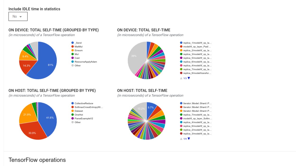
TensorFlow stats
The TensorFlow Stats tool displays the performance of every TensorFlow op (op) that is executed on the host or device during a profiling session.
The tool displays performance information in two panes:
-
The upper pane displays up to four pie charts:
- The distribution of self-execution time of each op on the host.
- The distribution of self-execution time of each op type on the host.
- The distribution of self-execution time of each op on the device.
- The distribution of self-execution time of each op type on the device.
-
The lower pane shows a table that reports data about TensorFlow ops with one row for each op and one column for each type of data (sort columns by clicking the heading of the column). Click the Export as CSV button on the right side of the upper pane to export the data from this table as a CSV file.
Note that:
- If any ops have child ops:
- The total "accumulated" time of an op includes the time spent inside the child ops.
- The total "self" time of an op does not include the time spent inside the child ops.
- If an op executes on the host:
- The percentage of the total self-time on device incurred by the op on will be 0.
- The cumulative percentage of the total self-time on device up to and including this op will be 0.
- If an op executes on the device:
- The percentage of the total self-time on host incurred by this op will be 0.
- The cumulative percentage of the total self-time on host up to and including this op will be 0.
- If any ops have child ops:
You can choose to include or exclude Idle time in the pie charts and table.
Trace viewer
The trace viewer displays a timeline that shows:
- Durations for the ops that were executed by your TensorFlow model
- Which part of the system (host or device) executed an op. Typically, the host executes input operations, preprocesses training data and transfers it to the device, while the device executes the actual model training
The trace viewer allows you to identify performance problems in your model, then take steps to resolve them. For example, at a high level, you can identify whether input or model training is taking the majority of the time. Drilling down, you can identify which ops take the longest to execute. Note that the trace viewer is limited to 1 million events per device.
Trace viewer interface
When you open the trace viewer, it appears displaying your most recent run:
This screen contains the following main elements:
- Timeline pane: Shows ops that the device and the host executed over time.
- Details pane: Shows additional information for ops selected in the Timeline pane.
The Timeline pane contains the following elements:
- Top bar: Contains various auxiliary controls.
- Time axis: Shows time relative to the beginning of the trace.
- Section and track labels: Each section contains multiple tracks and has a triangle on the left that you can click to expand and collapse the section. There is one section for every processing element in the system.
- Tool selector: Contains various tools for interacting with the trace viewer such as Zoom, Pan, Select, and Timing. Use the Timing tool to mark a time interval.
- Events: These show the time during which an op was executed or the duration of meta-events, such as training steps.
Sections and tracks
The trace viewer contains the following sections:
- One section for each device node, labeled with the number of the device chip and the device node within the chip (for example,
/device:GPU:0 (pid 0)). Each device node section contains the following tracks:- Step: Shows the duration of the training steps that were running on the device
- TensorFlow Ops: Shows the ops executed on the device
- XLA Ops: Shows XLA operations (ops) that ran on the device if XLA is the compiler used (each TensorFlow op is translated into one or several XLA ops. The XLA compiler translates the XLA ops into code that runs on the device).
- One section for threads running on the host machine's CPU, labeled "Host Threads". The section contains one track for each CPU thread. Note that you can ignore the information displayed alongside the section labels.
Events
Events within the timeline are displayed in different colors; the colors themselves have no specific meaning.
The trace viewer can also display traces of Python function calls in your TensorFlow program. If you use the tf.profiler.experimental.start API, you can enable Python tracing by using the ProfilerOptions namedtuple when starting profiling. Alternatively, if you use the sampling mode for profiling, you can select the level of tracing by using the dropdown options in the Capture Profiledialog.
GPU kernel stats
This tool shows performance statistics and the originating op for every GPU accelerated kernel.
The tool displays information in two panes:
- The upper pane displays a pie chart which shows the CUDA kernels that have the highest total time elapsed.
- The lower pane displays a table with the following data for each unique kernel-op pair:
- A rank in descending order of total elapsed GPU duration grouped by kernel-op pair.
- The name of the launched kernel.
- The number of GPU registers used by the kernel.
- The total size of shared (static + dynamic shared) memory used in bytes.
- The block dimension expressed as
blockDim.x, blockDim.y, blockDim.z. - The grid dimensions expressed as
gridDim.x, gridDim.y, gridDim.z. - Whether the op is eligible to use Tensor Cores.
- Whether the kernel contains Tensor Core instructions.
- The name of the op that launched this kernel.
- The number of occurrences of this kernel-op pair.
- The total elapsed GPU time in microseconds.
- The average elapsed GPU time in microseconds.
- The minimum elapsed GPU time in microseconds.
- The maximum elapsed GPU time in microseconds.
Memory profile tool
The Memory Profile tool monitors the memory usage of your device during the profiling interval. You can use this tool to:
- Debug out of memory (OOM) issues by pinpointing peak memory usage and the corresponding memory allocation to TensorFlow ops. You can also debug OOM issues that may arise when you run multi-tenancy inference.
- Debug memory fragmentation issues.
The memory profile tool displays data in three sections:
- Memory Profile Summary
- Memory Timeline Graph
- Memory Breakdown Table
Memory profile summary
This section displays a high-level summary of the memory profile of your TensorFlow program as shown below:
The memory profile summary has six fields:
-
Memory ID: Dropdown which lists all available device memory systems. Select the memory system you want to view from the dropdown.
-
#Allocation: The number of memory allocations made during the profiling interval.
-
#Deallocation: The number of memory deallocations in the profiling interval
-
Memory Capacity: The total capacity (in GiBs) of the memory system that you select.
-
Peak Heap Usage: The peak memory usage (in GiBs) since the model started running.
-
Peak Memory Usage: The peak memory usage (in GiBs) in the profiling interval. This field contains the following sub-fields:
- Timestamp: The timestamp of when the peak memory usage occurred on the Timeline Graph.
- Stack Reservation: Amount of memory reserved on the stack (in GiBs).
- Heap Allocation: Amount of memory allocated on the heap (in GiBs).
- Free Memory: Amount of free memory (in GiBs). The Memory Capacity is the sum total of the Stack Reservation, Heap Allocation, and Free Memory.
- Fragmentation: The percentage of fragmentation (lower is better). It is calculated as a percentage of
(1 - Size of the largest chunk of free memory / Total free memory).
Memory timeline graph
This section displays a plot of the memory usage (in GiBs) and the percentage of fragmentation versus time (in ms).
The X-axis represents the timeline (in ms) of the profiling interval. The Y-axis on the left represents the memory usage (in GiBs) and the Y-axis on the right represents the percentage of fragmentation. At each point in time on the X-axis, the total memory is broken down into three categories: stack (in red), heap (in orange), and free (in green). Hover over a specific timestamp to view the details about the memory allocation/deallocation events at that point like below:
The pop-up window displays the following information:
- timestamp(ms): The location of the selected event on the timeline.
- event: The type of event (allocation or deallocation).
- requested_size(GiBs): The amount of memory requested. This will be a negative number for deallocation events.
- allocation_size(GiBs): The actual amount of memory allocated. This will be a negative number for deallocation events.
- tf_op: The TensorFlow op that requests the allocation/deallocation.
- step_id: The training step in which this event occurred.
- region_type: The data entity type that this allocated memory is for. Possible values are
tempfor temporaries,outputfor activations and gradients, andpersist/dynamicfor weights and constants. - data_type: The tensor element type (e.g., uint8 for 8-bit unsigned integer).
- tensor_shape: The shape of the tensor being allocated/deallocated.
- memory_in_use(GiBs): The total memory that is in use at this point of time.\
Memory breakdown table
This table shows the active memory allocations at the point of peak memory usage in the profiling interval.
There is one row for each TensorFlow Op and each row has the following columns:
-
Op Name: The name of the TensorFlow op.
-
Allocation Size (GiBs): The total amount of memory allocated to this op.
-
Requested Size (GiBs): The total amount of memory requested for this op.
-
Occurrences: The number of allocations for this op.
-
Region type: The data entity type that this allocated memory is for. Possible values are
tempfor temporaries,outputfor activations and gradients, andpersist/dynamicfor weights and constants. -
Data type: The tensor element type.
-
Shape: The shape of the allocated tensors.
Note: You can sort any column in the table and also filter rows by op name.
Pod viewer
The Pod Viewer tool shows the breakdown of a training step across all workers.
- The upper pane has a slider for selecting the step number.
- The lower pane displays a stacked column chart. This is a high level view of broken down step-time categories placed atop one another. Each stacked column represents a unique worker.
- When you hover over a stacked column, the card on the left-hand side shows more details about the step breakdown.
tf.data bottleneck analysis
Warning: This tool is experimental. Please open a
The tf.data bottleneck analysis tool automatically detects bottlenecks in tf.data input pipelines in your program and provides recommendations on how to fix them. It works with any program using tf.data regardless of the platform (CPU/GPU/TPU). Its analysis and recommendations are based on this guide.
It detects a bottleneck by following these steps:
- Find the most input bound host.
- Find the slowest execution of a
tf.datainput pipeline. - Reconstruct the input pipeline graph from the profiler trace.
- Find the critical path in the input pipeline graph.
- Identify the slowest transformation on the critical path as a bottleneck.
The UI is divided into three sections: Performance Analysis Summary, Summary of All Input Pipelines and Input Pipeline Graph.
Performance analysis summary
This section provides the summary of the analysis. It reports on slow tf.data input pipelines detected in the profile. This section also shows the most input bound host and its slowest input pipeline with the max latency. Most importantly, it identifies which part of the input pipeline is the bottleneck and how to fix it. The bottleneck information is provided with the iterator type and its long name.
How to read tf.data iterator's long name
A long name is formatted as Iterator::<Dataset_1>::...::<Dataset_n>. In the long name, <Dataset_n> matches the iterator type and the other datasets in the long name represent downstream transformations.
For example, consider the following input pipeline dataset:
dataset = tf.data.Dataset.range(10).map(lambda x: x).repeat(2).batch(5)
The long names for the iterators from the above dataset will be:
|
Iterator Type |
Long Name |
|---|---|
|
Range |
Iterator::Batch::Repeat::Map::Range |
|
Map |
Iterator::Batch::Repeat::Map |
|
Repeat |
Iterator::Batch::Repeat |
|
Batch |
Iterator::Batch |
Summary of all input pipelines
This section provides the summary of all input pipelines across all hosts. Typically there is one input pipeline. When using the distribution strategy, there is one host input pipeline running the program's tf.data code and multiple device input pipelines retrieving data from the host input pipeline and transferring it to the devices.
For each input pipeline, it shows the statistics of its execution time. A call is counted as slow if it takes longer than 50 μs.
Input pipeline graph
This section shows the input pipeline graph with the execution time information. You can use "Host" and "Input Pipeline" to choose which host and input pipeline to see. Executions of the input pipeline are sorted by the execution time in descending order which you can choose using the Rank dropdown.
The nodes on the critical path have bold outlines. The bottleneck node, which is the node with the longest self time on the critical path, has a red outline. The other non-critical nodes have gray dashed outlines.
In each node,Start Time indicates the start time of the execution. The same node may be executed multiple times, for example, if there is a Batch op in the input pipeline. If it is executed multiple times, it is the start time of the first execution.
Total Duration is the wall time of the execution. If it is executed multiple times, it is the sum of the wall times of all executions.
Self Time is Total Time without the overlapped time with its immediate child nodes.
"# Calls" is the number of times the input pipeline is executed.
Originally published on the