Table of Links
-
Introduction
1.1 Periodic auction and continuous limit order book
1.2 Comparison and main flaws of limit order book
1.3 Optimal policies to cure auction’s inefficiencies and related works
-
Auctions market modeling with transaction fees and randomization
2.1 The market characteristics
2.3 Strategic Trader’s optimization and market quality
2.4 Data and numerical analysis
2.5 Strategic trader with full information: efficient but unfair market
-
Monitoring policies: transaction fees and clearing time randomization
3.1 Bilevel optimization between the exchange and the strategic trader
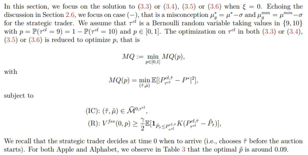
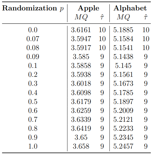
3.2 Randomization without fees
3.3 Optimal transaction fees indexed on time to improve price impact for the trader
A. Appendix: Numerical Methods
A.1 Problem of a Strategic Seller
A.2 Appendix: Problem of the Regulator
B Appendix: Illustrate Remark 2.4
3.1 Bilevel optimization between the exchange and the strategic trader
where[8]
Remark 3.1. This problem can by also seen as a “trader focused” exchange. We assume the exchange wants to minimize the total spread for the trader, where
total spread =MQ + transaction spread
= spread between efficient price and clearing price+
spread between clearing price and after-fee price (real executed price).

If the exchange focuses only on the market efficiency and wants to increase both fee gains and market quality, the problem becomes
Remark 3.2. Note that for both market impact or market efficiency optimization problems, we focus solely on the spread and fee of the strategic trader. We do not include the spread and fee of the other transferred limit orders because we assume these traders are transferred from CLOB to the periodic auction for execution and thus do not face the transaction fee imposed in the periodic auction.
3.2 Randomization without fees
3.3 Optimal transaction fees indexed on time to improve price impact for the trader
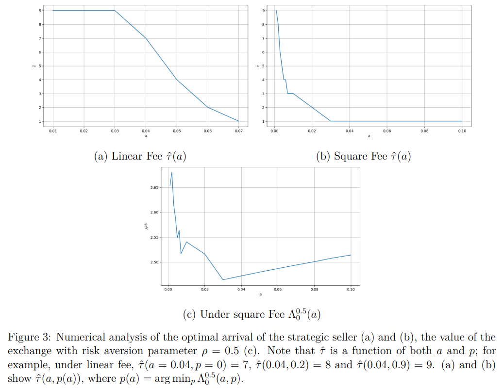
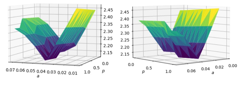
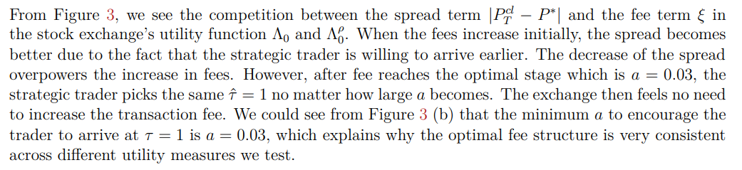
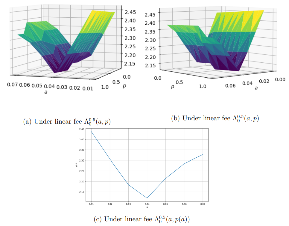
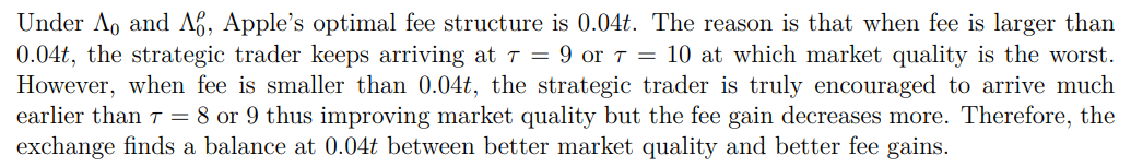
We now turn to a deeper study of how our transaction fee model improves the market’s quality for the Apple’s stock price.[9] Both the linear transaction fee structure and square transaction fee structure encourage the strategic seller to arrive earlier in the market. From Figure 3 (a) and (b), we see that as the fee increases (led by increasing a), the strategic seller’s optimal τ gradually declines from 10 to 1 and the decline rate seems to coincide with the structure of the fee model as Figure 3 (a) shows a linear declining pattern and Figure 3 (b) shows an accelerating declining pattern.
3.4 Optimal transaction fees indexed on time: improving market quality while benefiting from the fees
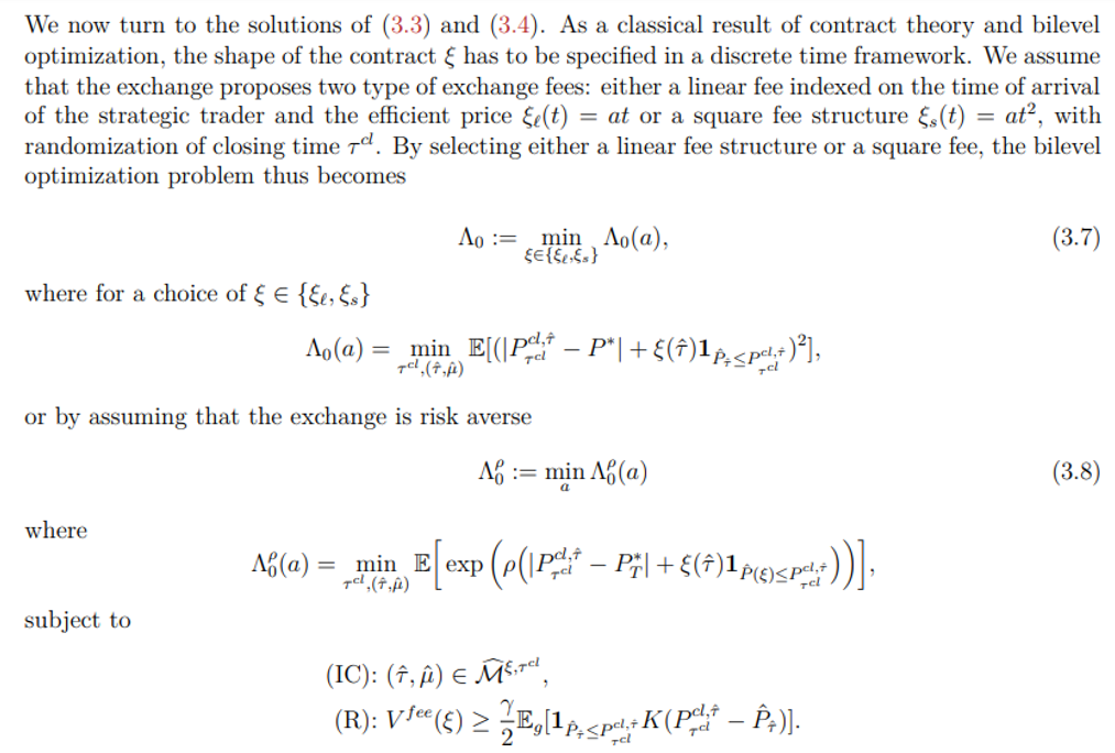
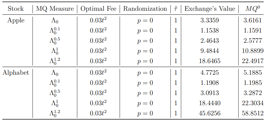
We now turn to the solutions of (3.5) and (3.6). The bilevel optimization problem thus becomes
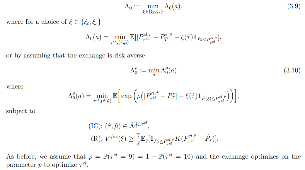
Remark 3.3. In an informal way, we can see from (3.9) or (3.10) that
Exchange value function = market quality cost − fees,
or in other words
Market quality cost = Exchange gain + Fees’ gain.
Authors:
(1) Thibaut Mastrolia, UC Berkeley, Department of Industrial Engineering and Operations Research (thibaut.mastrolia@berkeley.edu);
(2) Tianrui Xu, UC Berkeley, Department of Mathematics (tianrui.xu@berkeley.edu).
This paper is

[story continues]
tags