Potholes, Pipelines, and Precision: Benchmarking Object Detectors for Global Road Safety

Table of Links

Abstract and I. Introduction

II. Dataset

III. Methods

IV. Experiments

V. Results

VI. Conclusions and References

III. METHODS

There are two main classes of object detectors that are consistently performing well on the popular Microsoft Common Objects in Context (MS COCO) [6] dataset. In one-stage detection it is YOLO [13], RetinaNet [7] and in two-stage region proposal based Faster R-CNN [4] or Mask R-CNN [8] methods are widely used. Mask R-CNN is an extension of Faster R-CNN with an additional mask proposal branch for segmentation.

YOLO has a single neural network that predicts bounding boxes and class probabilities directly from full images in one evaluation. Since the whole detection pipeline is a single network, it can be optimized end-to-end directly on detection performance.

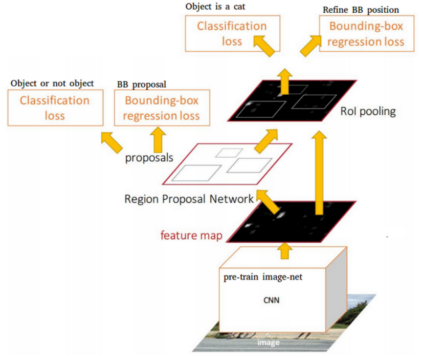
Faster R-CNN [4] is a region based approaches that predicts detections based on features from a local region. This region is localized using a Region Proposal Network (RPN). The first stage network is for region proposal on the features from convolution backbone and the second stage is a fully connected network for object classification and bounding box regression.

A. Convolution Backbone

The backbone network is a standard Convolutional Neural Networks (CNN), used to extract high level visual features from the entire image. The high level features are represented as convolutional feature map over the image. Deep Residual Networks [9] like Resnet 50, Resnet 101, ResneXt 101 and Feature Pyramid Network (FPN) or a combination of Resnet and FPN have shown to work well with most object detection models including Faster R-CNN and Mask R-CNN.

One-stage networks like RetinaNet have also used Residual Network and FPN based backbones. YoloV5 on the other hand have made use of Cross Stage Partial Network (CSPNet) [16] to achieve high benchmark on MS COCO datasets.

B. One Stage Object Detector

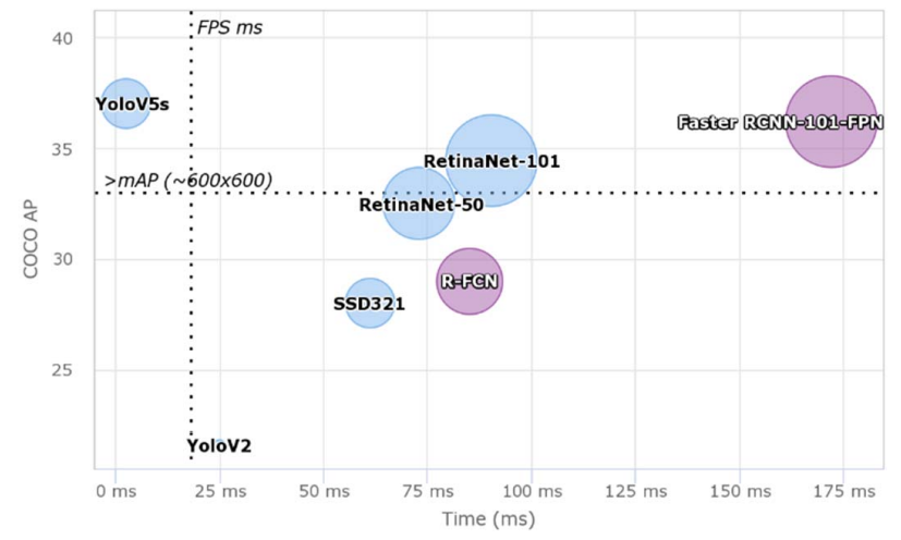
Yolo [13] and RetinaNet [7] are popular one-stage object detection models. The accuracy charts are typically lead by two-stage object detectors, whereas one stage detectors are preferred for evaluation speed. One stage detector tends to have low compute requirements and can be easily deployed on smartphone devices.

Yolo

You-Only-Look-Once (Yolo) [13] is a unified, real-time object detection algorithm that reformulates the object detection task to a single regression problem.

Yolo employs a single neural network architecture to predict bounding boxes and class probabilities directly from full images. When compared to Faster R-CNN, Yolo provides faster detection with the accuracy trade-off. This has been the core reason for its popularity and multiple extensions and adaptations like Yolov3 [13] and Yolov5 [15] have emerged from it.

Yolov5 [15] includes four different models ranging from the smallest Yolo-v5s with 7.5 million parameters (plain 7 MB and MS COCO pre-trained 14 MB) and 140 layers to the largest Yolo-v5x with 89 million parameters and 284 layers (plain 85 MB and MS COCO pre-trained 170 MB). In the approach considered in this paper, we have experimented with all 4 variants of Yolov5 models. It uses a two-stage detector that consists of a Cross Stage Partial Network (CSPNet) [16] backbone trained on MS COCO [6].

Each Bottleneck CSP unit consists of two convolutional layers with 1 × 1 and 3 × 3 filters. The backbone incorporates a Spatial Pyramid Pooling network (SSP) [17], which allows for dynamic input image size and is robust against object deformations.

C. Two Stage Object Detector

Region based CNN (R-CNN) serve as a class of object detection model which falls under two-stage detectors. Faster R-CNN is a region based approach that predicts detections based on features from a proposed region.

Faster R-CNN

Region proposal based detectors like Faster R-CNN [4] is a popular two-stage detectors. The first stage generates a sparse set of candidate objects using a Region Pooling Network (RPN), based on shared feature maps, this is classified as foreground or background class. The size of each anchor is configured using hyperparameters. Then, the proposals are used in the region of interest pooling layer (RoI pooling) to generate subfeature maps. The subfeature maps are converted to 4096 dimensional vectors and fed forward into fully connected layers. These layers are then used as a regression network to predict bounding box offsets, with a classification network used to predict the class label of each bounding box proposal.

Feature Pyramid Network (FPN) [5] is employed as the backbone of the network. FPN uses a top-down architecture with lateral connections to build an in-network feature pyramid from a single-scale input. Faster R-CNN with an FPN backbone extracts RoI features from different levels of the feature pyramid according to their scale, but otherwise the rest of the approach is similar to vanilla Resnet. We also employ ResNeXt101 [20] with the FPN feature extraction backbone to extract the features.

IV. EXPERIMENTS

In this section, we evaluate one-stage Yolo v5 [15] and twostage Faster R-CNN [4] network with varied pre-processing, backbone network, hyper-parameter tuning and training strategy to achieve better Avg F1 score. We do not use ensemble approach considering that is great for competitions but rarely works well when deployed. In our backbone and methods, we have used Resnet 50, Resnet 101, ResneXt 101 [9, 20] and CSPNet [16] for evaluations considering that when trained these weights can be pruned and compressed to work on smaller devices with minor degradation in accuracy.

In our experiment we start with data pre-processing where we used image augmentation like resize, orientation, and DeepLab V3+ [18] based segmentation to isolate the road surface for downstream assessment.

Next, we look at training a detection model for each country and look at their performance on the submitted F1 score. We also train a single model with the data for all the three countries as a generalized approach. We focus more on the generalized approach considering the theme of this work and the challenge [23] is to obtain a model that can be transferred to other countries.

Finally, we look at thresholding and proposal ranking method applied to the detection results over test datasets. This is important as the output that we submit to the challenge should be the top proposals.

A PyTorch and Detectron2 [14] based framework from Facebook AI Research (FAIR) was used to train and evaluate the Faster R-CNN [4] models while a PyTorch based Yolov5 [15] implementation was used from Ultralytics for comparison purposes. All these implementations are available in opensource Github repository for the community. We were able to customize the data loader and mapper objects to setup the codebase for experimentation. Both these codebases support Tensorboard project for tracking the training accuracy and optimization loss throughout the training process.

The experiments reported in the various tables next, have the model description with epoch runs and chosen backbone network in the first column. Hyper-parameters are described in the second column. Average F1 score is reported for Test 1 and Test 2 dataset based on the kind of experiment we ran.

A. Pre-processing Images

We looked at segmentation as a way to eliminate background and noise from the image so that we can analyze features only on the road. A PyTorch and Detectron2 [14] based DeepLab V3+ [18] implementation is used for segmentation contours and image cropping.

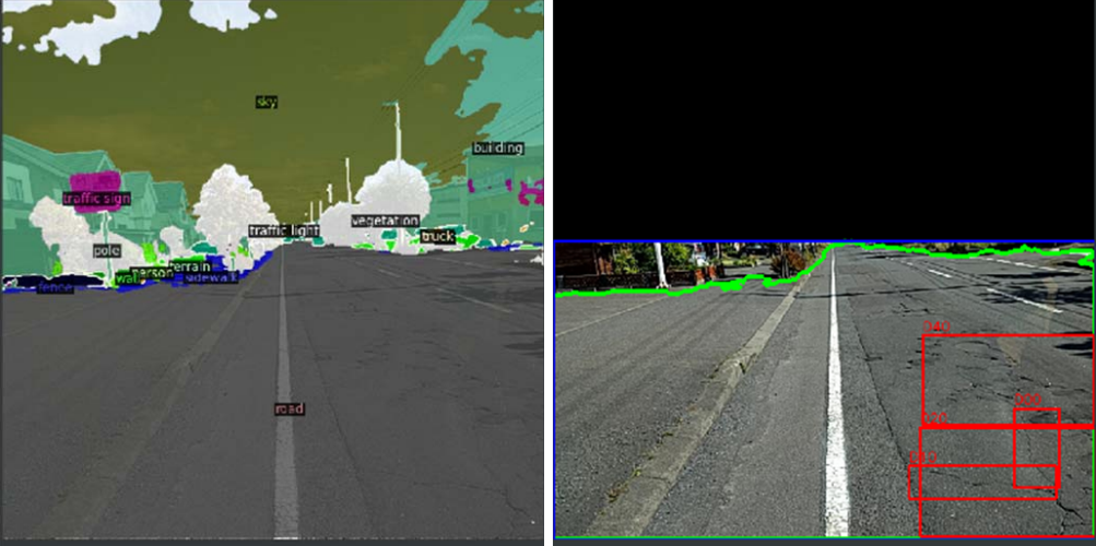
We used standard DeepLab V3+ [18] model trained on Cityscape semantic segmentation dataset. The model was able to achieve fair segmentation on most roads in Japan and Czech, while roads in India which had gravel and mud like surface, it did not do a good job of separating the road from surrounding surfaces. We did a basic analysis in Table II to verify, whether segmentation offered an improvement. The dataset used all countries annotation to train a single Faster R-CNN [4] model.

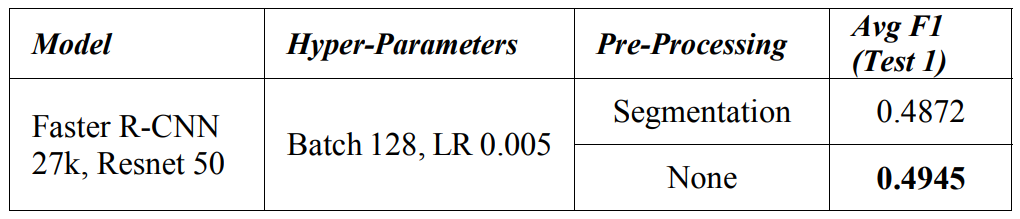
In our experiments, we did not observe any benefit based on our segmentation approach. It appears that the model performance deteriorates and that could stem from segmentation in the India dataset. We proceed without segmentation for the rest of the dataset pre-processing.

B. Model per country

We trained Faster R-CNN [4] models to fit the data of each country in order to achieve the baseline. The expectation was that the model will achieve better accuracy with three different models dedicated to Czech, Japan and India. We look at a comparison of this approach in Table III.

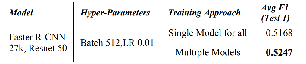
We get a 1.5% benefit in Average F1 score metric when we train with the baseline Train/Val (T) dataset. However, we take the approach of training a single model across the country’s dataset considering the benefits of deployment and model management.

C. Generalized Model

We attempt to generalize the model by training it on the data from all the countries in the dataset. Here we attempt to compare the two-stage Faster R-CNN [4] and one-stage YoloV5 [15] detection models. We clearly observe in Table IV that two-stage detector out-performs the one-stage detector.

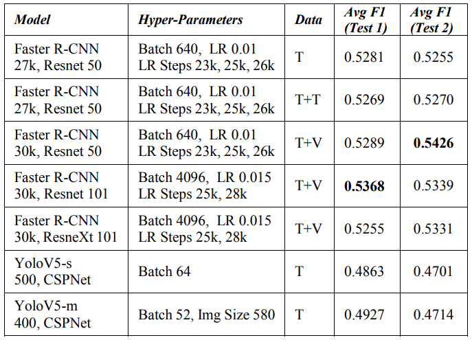
The data used in training these models consists of Train/Val (T) baseline split that is described in the dataset section. We combine Train and Test (T+T) data for training for the second set in the table. Thereafter we improve upon this by composing Train and Val (T+V) data for training the remaining Faster RCNN model runs. We do gain the expected benefit with this data composition.

The Model description in Table IV consists of the model name, epoch runs and backbone network. We observe that Faster R-CNN model performs better than YoloV5. The Hyperparameters includes Batch size, Learning Rate (LR) and LR Step Scheduler. A scheduler decreases the LR by a gamma factor of 0.05 over the steps of mentioned epoch values. LR of 0.01 and 0.015 have performed well with a step schedule of (23k, 25k, 26k) and (25k, 28k) epochs respectively.

We show the best F1 score in Table IV for Faster R-CNN [4] based on a batch size 640 and Resnet 50 [9] in Test 2 evaluation while for Test 1 evaluation score web observe Batch size 4096 and Resnet 101 [9] seems to work well.

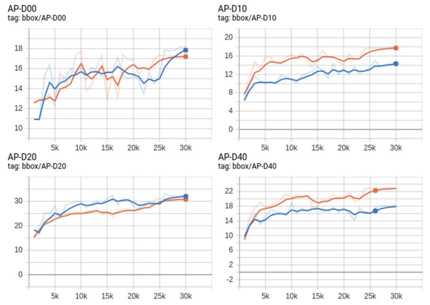
We look at the mean accuracy (IoU=.50:.05:.95) on the 5% split Test (T) dataset to monitor and track the progress of the models training. We see in Fig. 8, that this dataset shows high bounding box accuracy on D20 damage type in both the models. However, Resnet 50 with Batch 640 trained model seems to perform well on D10 and D40 damage types, considering both of those classes have relatively low annotations.

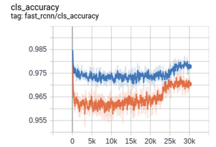
When we look at damage classification accuracy in Fig. 9, the Resnet 101 [9] backbone with high batch size demonstrates high accuracies. We also see that the LR step scheduler has a significant impact on the accuracy around 23k for the smaller network and around 25k for the larger network. We also see that the model stops learning around 30k epoch and an early stopping method is used to end the training process. This stops the model from overfitting the training data.

A generalized approach with low network size may allow the model to transfer across countries and reduce the deployment overhead based on the target conditions. However, a bigger network has higher classification accuracy.

D. Post-processing

In this step we look at operations after detection. The resulting bounding boxes are filtered at 0.7 confidence threshold. Additionally, the detections are sorted by confidence and only the top 5 bounding boxes are sampled for best submission.