PreCorrector Proves Its Worth: Classical Preconditioners Meet Their Neural Match

Table of Links

Abstract and 1 Introduction

2 Neural design of preconditioner

3 Learn correction for ILU and 3.1 Graph neural network with preserving sparsity pattern

3.2 PreCorrector

4 Dataset

5 Experiments

5.1 Experiment environment and 5.2 Comparison with classical preconditioners

5.3 Loss function

5.4 Generalization to different grids and datasets

6 Related work

7 Conclusion and further work, and References

Appendix

5 Experiments

In our approach, we use both IC(0) and ICt(1) as starting points for training. In the next section, we will use following notations:

• IC(0), ICt(1), ICt(5) are classical preconditioners from linear algebra with a corresponding level of fill-in k.

• PreCorrector IC(0) and PreCorrector ICt(1) are the proposed approach with corresponding preconditioner as input

5.1 Experiment environment

5.2 Comparison with classical preconditioners

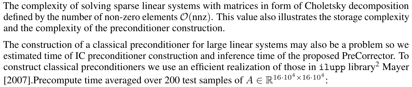
The proposed approach construct better preconditioner with increasing complexity of linear systems (Table 1). As the variance and/or grid size of the dataset grows, PreCorrector IC(0) preconditioner, made with IC(0) sparsity pattern, outperform the same vanilla preconditioner up to a factor of 3. This effect is particularly important for memory/efficiency trade-off. If one can afford memory, the PreCorrector ICt(1) preconditioner produces speed-up up to a factor of 2 compared to ICt(1).

While it is not completely fair to compare results of preconditioners with different densities, we observed that PreCorrector can outperform classical preconditioners with greater nnz values. The PreCorrector IC(0) outperform ICt(1) up to a factor of 1.2 − 1.5, meaning we can achieve better approximation P ≈ A with less nnz value. Moreover, the effect of the PreCorrector ICt(1) preconditioner is comparable to the ICt(5) preconditioner, which has 1.5 times larger nnz value than initial matrix A (A.2.

Architecture of the PreCorrector opens for interpretations value of the correction coefficient α in (6). In our experiments, the value of α is always negative and its values are clustered in intervals [−0.135, −0.095] and [−0.08, −0.04]. One can find greater details about values of coefficient α in Appendix A.3.

5.3 Loss function

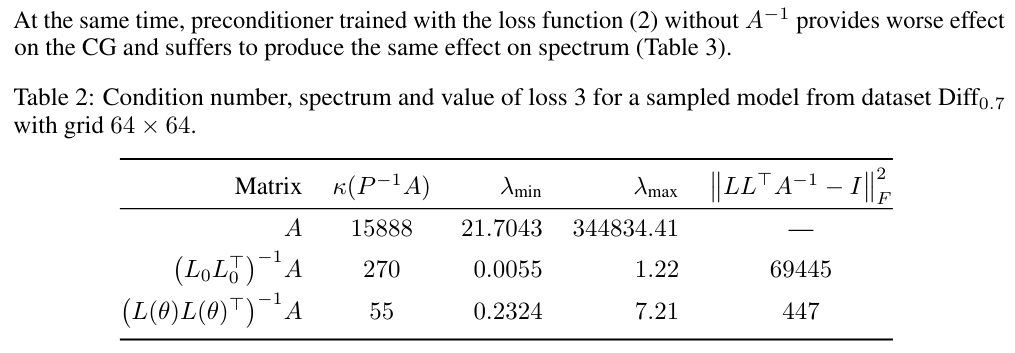
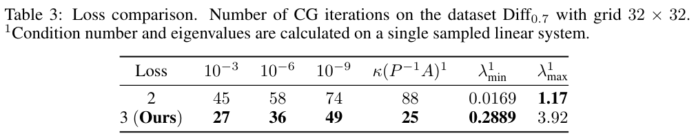
As stated in Section 2, one should focus on approximation of low frequency components. In the Table 2 we can see that the proposed loss does indeed reduce the distance between extreme eigenvalues compared to IC(0). Moreover, the gap between the extreme eigenvalues is covered by the increase in the minimum eigenvalue, which supports the hypothesis of low frequency cancellation. Maximum eigenvalue also grows but with way less order of magnitude.

5.4 Generalization to different grids and dataset

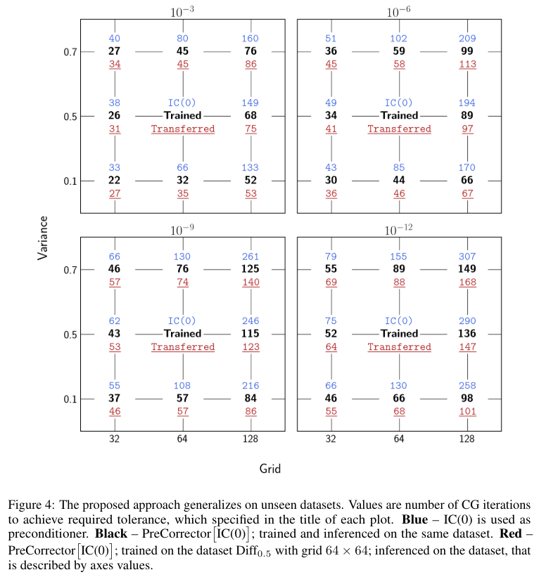
We also observe a good generalization of our approach when transferring our preconditioner between grids and datasets (Figure 4). The transfer between datasets of increasing and decreasing complexity does not lead to a loss of quality. This means that we can train the model with simple PDEs and then use it with complex ones for inference. If we fix the complexity of the dataset and try to transfer the learned model to other grids, we observe a loss of quality of only about 10%.

[2] https://github.com/c-f-h/ilup