Tape Isn’t Slow, Pipelines Are

How to Orchestrate Multiple Tape Libraries and Media Pools for Recalls

Everyone “knows” tape is slow. That’s cute. Tape is a streaming device that will happily shovel data until your pipeline chokes on something human-made: a queue that lies, a scheduler that panic-mounts, or a drive fleet that’s treated like a bottomless piñata. If your recall plan is “open the firehose and pray,” you don’t have a plan—you have a mount storm.

This piece discusses how you run multiple tape libraries and media pools like adults: VSN-driven recalls, mount/seek realities, drive sharing, sane concurrency, ACSLS recovery tactics, and queue hygiene. I’ll keep the snark sprinkled in to keep the eyes un-glazed; consider it the caffeine your Gantt chart forgot.

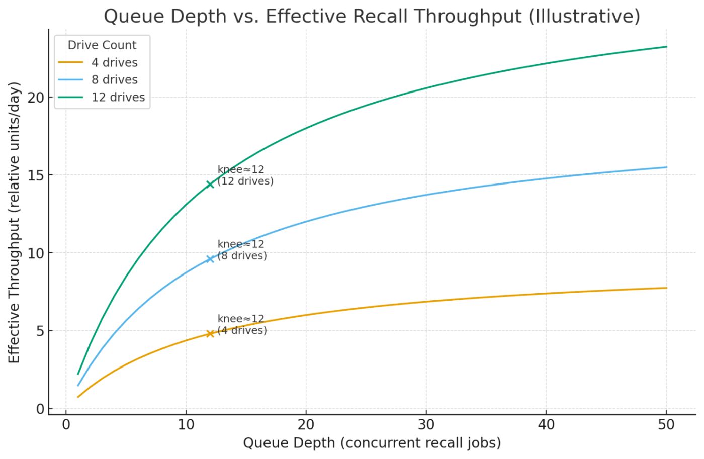
(Grab the visual: Queue Depth vs. Effective Recall Throughput with drive-count curves. It’s illustrative, but it’ll stop three arguments in your next war room.)

First principles your pipeline forgot

Tape streams; humans seek. Tape is happiest when you ask for long, sequential reads. It gets grumpy when you demand lottery access across millions of small files. That “grumpy” shows up as shoe-shining (back-and-forth repositioning) and your “95 MB/s per drive” magically becomes “is it… moving?”

Drives are not throughput; pipelines are. Your effective recall rate is the minimum of: staging, verify, transfer, ingest, and post-write verify. The fast part doesn’t matter if the slowest part is slow. (Yes, this is the sequel to “Calculators Lie, Queues Don’t.”)

Libraries are ecosystems, not vending machines. Each one has its own picker personality, import/export cadence, drive firmware quirks, and “that one slot bank” everyone side-eyes. You are orchestrating ecosystems—not issuing mt -f incantations into the void.

VSN-driven recalls: make physics your friend

A VSN (volume serial number) is more than a barcode—it’s a batching hint. You want your scheduler to express intent at the VSN level, not whack-a-file across 200 tapes.

Rules of engagement:

Batch by VSN and class:

• Guarantee day-mix per drive bank: e.g., 1×S : 5×L at any moment. Two S tapes in the same hour per drive is how ops becomes stand-up comedy.
• Pin VSNs to drive groups when you can. A single Class S on a drive can occupy it far longer than a Class L. You want predictable occupancy, not surprise hostage situations.

Why VSN batching beats filename batching: you’re optimizing for mounts and seek behavior, not for your favorite prefix. Tape doesn’t care about your directory tree; it cares about physics.

Mount/seek realities: the shoe-shine bill you didn’t pay

Let’s show junior admins why the old-timers mutter about shoe-shining.

Back-of-envelope:

• N_files = number of files on the tape
• S_avg = average file size (GiB)
• B_stream = streaming bandwidth (GiB/s) when happy
• L_seek = average per-file positioning latency (s)

TotalSizeGiB = N_files * S_avg
StreamingTime = TotalSizeGiB / B_stream
SeekTime      = N_files * L_seek
TotalTime     = SeekTime + StreamingTime

If N_files is in the millions and L_seek is seconds (it usually is), SeekTime dominates. Your “it’s only 12 GB” tape becomes a multi-day therapy session. The antidote is classing + batching + not letting small-file tapes flood the day.

Drive sharing reality: 12 drives does not mean 12× speed when half your day’s VSNs are small-file tarballs. On small-file workloads the effective per-drive output can fall two orders of magnitude vs. spec. Don’t schedule to spec; schedule to classed reality.

Concurrency patterns: how to go fast without eating your own queue

Use the plot you downloaded. It’s an illustrative saturation curve: throughput increases with queue depth until the knee, then flattens and eventually declines as you thrash pickers, mounts, and operator attention.

Practical defaults (tune per fleet):

• Knee heuristic: knee ≈ 1× to 2× the number of drives per library for Class L days; knee ≈ 0.5× drives for Class S days.

• Mount budget: cap to ≤ 6 mounts/hour/drive sustained. More looks busy; it’s actually slow.

• Queue admits: don’t let more work in than the slowest downstream can drain (min(R_stage, R_verify, R_ingest)). Backpressure early; the goal is steady streaming, not “CPU graphs that look like cardiograms.”

  Sharing drives across pools:

• Priority pools: Give preservation “deadline” VSNs pre-emptive rights only if the scheduler can pre-commit mounts; otherwise you’ll be mid-stream starving.

• Fairness window: slice time by N-minute quanta per pool (e.g., 20-minute windows), not file count. Time slices respect tape physics; file counts lie.

ACSLS recovery tactics: how not to recreate 2009

When (not if) ACSLS loses its marbles:

Golden triage:

• Single-fault rollback before you shoot the cluster. Half the pain comes from “fix everything” runs that break healthy ACSs.
• Inventory quarantine: mark suspect slots/VSNs “no-queue” until reconciled; do not let the scheduler “try anyway.”
• Pick-count budget: configure a max picks/hour per library during recovery—your operators have finite hands and caffeine.

Snarky but true: if your recovery runbook starts with “restart all the things,” it’s not a runbook; it’s a ritual.

Queue hygiene: how grown-ups keep throughput boring (the good kind)

• Poison-pill protocol: any file/VSN that fails N times goes to quarantine with context (drive, slot, error text). The mainline queue never blocks behind a diva.
• Idempotent writes: destination paths must tolerate retries without duplicates; if your ingest can create zombie objects, your queue will.
• Admit control: rate-limit enqueues to the slowest concrete stage over the last hour (EWMA). “Full queue” is not a KPI.
• Mount bundling: round up same-VSN requests every t seconds so you ride a single mount longer. If your scheduler trickles 100 tiny jobs across 10 VSNs, that’s your throughput you hear crying.
• Drive hygiene: proactive clean cycles and firmware windows scheduled against small-file days; don’t take five drives out of service when you already told physics you were going to win.

Drive sharing: when you have more libraries than patience

If you run multi-library, multi-pool:

• Pool-to-library affinity with escape hatches. You want your queue to prefer home libraries (cache locality, picker path), but allow spillover when the home pool saturates and the target has free drives.
• Picker locality awareness: some libraries are marathoners; some are sprinters. Put Class S near sprinters—they’ll waste less time between short seeks.
• Cross-lib fairness: never let one library starve because a neighbor is constantly at 99% mounts/hour; reserve a minimum drive floor per library (e.g., “≥2 drives always available”).

Teaching the juniors: the mental model you want them to have

“Streaming good, seeking expensive.” Long reads good. Micro-jumps bad. If your Grafana shows mounts climbing and throughput flat, you’re seeking, not streaming.

“Mounts are currency.” Spend mounts on batches, not on hope. Mount budgets, mount bundling, mount floors—these are throughput knobs, not bureaucracy.

“Queues lie if you let them.” A fat queue is not progress; it’s pressure. Your goal is smooth, knee-aware flow. Show them the saturation plot and the knee; make “past the knee” a smell they can recognize.

“APS (Always Pick Sane).” Given two VSNs, pick the one that increases sequentiality. The best junior admins learn to spot streaming opportunities by filename patterns and VSN metadata, not “which request came first.”

Numbers and signals to run by (copy/paste into your SLO doc)

• Mounts/hour/drive (target ≤ 6 sustained; warn at 8)
• Sequentiality ratio per drive: bytes streamed / bytes read (the closer to 1, the happier the tape)
• VSN class mix per hour (S:L ratio)
• Queue age (P95) per class
• Drive unavailability (sum of clean + fault + fw) vs. schedule
• Picker travel time (median + P95); rising == you’re thrashing slots
• Recall to verify lag (minutes); if verify can’t keep up, you’re building verification debt
• Abort/retry rate by error family (media, drive, path, scheduler)

A tiny bit of math (and a big explanatory payoff)

Use this compact model to size day plans and talk to management without a three-hour seminar:

Let:
  D = number of active drives
  q = queue depth (concurrent recall jobs)
  sat = knee parameter (empirical; ~ D for L-days; ~ 0.5*D for S-days)
  K = per-drive streaming capacity (relative units/day)

EffectiveThroughput(q, D) ≈ D * (q / (q + sat)) * K

• When q << sat: you’re under-feeding the drives; throughput rises with q.
• Around q ≈ sat: you’ve hit the knee; each extra job adds less than you think.
• When q >> sat: picker/mount thrash; your efficiency falls while ops slacks explode.

Your action item for juniors: find today’s knee and keep q near it, not past it. (Yes, managers love this sentence. Yes, you should put it on a mug.)

ACSLS “oh no” runbook (copy/paste)

1. Freeze admits to the affected library.
2. Health triage: drive map, picker status, volatile logs, inventory spot check (10 random slots/VSNs).
3. Quarantine any VSN with inconsistent location, do not auto-retry.
4. Reduce mounts/hour by 50% for 60 minutes; allow in-flight streams to drain.
5. Selective service restarts (one component at a time) with logs tailed and a witness.
6. Inventory reconcile (delta, not full scan).
7. Slow thaw admits with Class L first; re-enable S after one hour of clean runs.
8. Post-mortem: add this failure signature to the poison-pill list and update the no-queue mask.

If your current SOP says “restart everything and hope,” you deserve the 3 a.m. wake up call.

Putting it together: a day plan that doesn’t page itself

• Declare class mix: “Today: 80% L, 20% S.”
• Set knee: drives per lib = 8 → knee ~ 8 (L-heavy).
• Queue admits: cap q around 8–10 per lib; auto-backpressure on verify lag or ingest back-pressure.
• Mount budget: ≤ 6/hour/drive; bundling interval 90s to capture trickle.
• Drive floors: 2 per library reserved for priority pool.
• ACSLS watch: pick-count limit and inventory drift alarms armed.
• Metrics board: mounts/hour, sequentiality ratio, recall→verify lag, queue age P95, abort rate, drive unavailability.
• People: one operator per 6–8 drives during S-heavy windows; otherwise 1 per 12 is survivable with good dashboards.

One tasteful snark (because engagement is a feature)

If your recall plan is “throw more jobs at it until throughput happens,” I have great news: congratulations on inventing MountCoin—it burns energy, makes noise, and produces approximately nothing of value.

CTA

Where does your recall actually stall—mount storms, seek-bound S tapes, ACSLS wobble, or verify lag? If I dropped 10 random VSNs on your queue right now, could you tell me your knee and mount budget without opening Slack? Share the war story (names optional). I’ll trade you a knee-finder checklist and a mount-bundling script stub.