The Delicate Math Behind Prompt Compression and Profit Margins in LLMs

Table of Links

Abstract and 1. Introduction

2. Basic premises for our models

   2.1. How LLMs are charged

   2.2 An anedotal model from industry

   2.3 Choice of Costs in the Model

   2.4 Why multiple scenarios

3. A Decision Theoretic Model

   3.1 How to model success

4. A Model for Commercial Operations Based on a Single Transaction

   4.1 Example of Using the Model

   4.2 Model Analysis

   4.3 Discussion of the RoI vs. Earning dillema

5. Modelling of a Binary Classification Problem

   5.1 Local Sensitivity Analysis

   5.2 Global Sensitivity Analysis by Sobol Method

6. Related Work

7. Future work

8. Conclusion, References, and Acknowledgements

4.2 Model Analysis

We must point out that due to the use of LLM in a commercial context, the uncertainties will be mainly in G, L, and P. It would be reasonable to expect a normal probability distribution for P and a normal or even power probability distribution for G and L. Since G and L are business values, and P is the business result that comes from performing the AI tasks correctly, these values are not under the direct control of the project team. We recall that a complete model of the probability of success should start from Equation 17, but this is beyond the scope of this article.

On the other hand, T, that is, the size of the transaction in tokens, it is more under the control of the project team, since it depends on the size of data used, and desired, at input and output, and also the size of the prompt. One should also expect a normal or power probability distribution for T. Finally, for a single LLM chosen, C is actually a constant, and we only need to understand its impact on the decision when more than one LLM is considered.

Looking at Equation 18, we can also see that if G and L are large and T small, the factor CT will be small and E[E] will be mainly a function of GP −L(1−P), and since G and P are expected to have the same distribution for a single business task, P would have the greater impact. This could greatly impact the evaluation of prompt compression techniques, such as LLMLinguaJiang et al. [2023a,b], Pan et al. [2024] for small prompts. For example, suppose that a classification task using a 1,000 token transaction could result in US$10 gain or US$1 loss. Its cost would be US$0.005 in GPT 4o. Therefore, compressing the prompt 20× would save US$0.00475 in CT. Meanwhile, each 1% lost in P would result in a GP − L(1 − P) loss of US$0.11. At the other hand, for small G and L, and larger T, compression could be effective.

Taking all this into account, we decided to perform both a local and a global sensitivity analysis to understand the impact of the parameters in E[E] and E[R]. We understand that the local sensitivity is easier to understand and reasonable in this case, while the global sensitivity is theoretically stronger; therefore, we also analyze the linearity of the functions to understand how valid the local analysis is.

4.2.1 Local Sensitivity Analysis

This first sensitivity analysis is local and qualitative. It is carried out by evaluating the partial derivatives of E[E] in relation to each variable in their respective intervals. This provides insight into how sensitive E[E] is to changes in each parameter within the ranges of variation.

Taking into account Equation 18, it is possible to find all the partial derivatives for variables G, C, T, P and L.

The partial derivatives for E[E] are:

The Hessian of E[E] is mostly composed of zeros, indicating a fairly linear behavior that would be very acceptable for a local analysis.

Similarly, the partial derivatives for E[R] are:

Thus, the Hessian matrix H of E[R] with respect to variables G, C, T, L, and P is:

The Hessian matrix of E[R] has fewer zeros, and the small value of C, found in the denominator of most partial derivatives, will bring greater values. This reflection is a challenge for local sensitivity analysis; however, looking at the partial derivatives still allows for some advantages on interpretability.

4.2.2 Global Sensitivity analysis of earnings by Sobol technique

Although local sensitivity analysis looks at one variable at each time in the neighborhood of a point, and thus is only adequate, if so, for linear and mostly linear functions, global analysis can study the effect of all variables at the same time, for specific distributions, even in the case of nonlinearity [Saltelli et al., 2004, 2008].

Sobol [2001] proposed a method for global sensitivity analysis based on running a model with a sampling generated under certain premises, and make a variance decomposition that allow the calculation of a set of indexes of sensitivity.

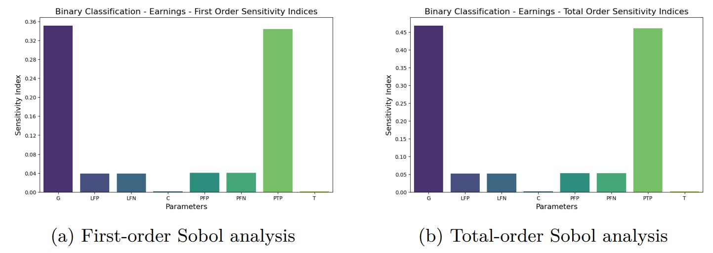
The first-order Sobol index measures the individual contribution of each input variable to the variance in the model output, ignoring interactions with other variables. In simpler terms, it quantifies how much of the uncertainty in the model output can be directly attributed to changes in a specific input, while all other inputs are held fixed. This quantification is performed between values 0 and 1 [Sobol, 2001].

The total order Sobol index quantifies the overall contribution of an input variable to the output variance, considering both its individual effect and its interactions with other variables. Essentially, it measures the impact of a variable on the output by accounting for all possible ways in which it can influence the result, including its combined effects with other variables. This index also ranges between values 0 and 1, indicating the proportion of output variability attributed to the total influence of the given input variable [Sobol, 2001].

Finally, the second-order, and higher orders, Sobol index is an extension of the first-order index and is used to measure the combined effect or interaction between pairs, or tuples, of input variables on the variance of the model output. While the first-order index focuses on the individual contribution of each variable, the second-order index examines how the interaction between two variables contributes to uncertainty in the output, beyond what would be expected based on the individual effects of each variable [Sobol, 2001]. This allows for a good visual representation of the combined effect of pair of variables in a matrix.

From the global sensitivity analysis of the earnings for the commercial operation model, it can be seen that the value of P is clearly the most important factor in the first order analysis Figure 2a. For the total order index, Figure 2b shows the importance of C and T, which is also reflected in the second order values, shown in Figure 3, which shows the clear predominance of the pair C and T as a pair. The product CT is the total cost of the transaction.

The RoI sensitivity analysis for the commercial operation model shows that RoI is particularly sensitive to changes C, T and P for the total order, within the given ranges. In particular, the combination of C and T has the greater impact on the variation of RoI of the second order. Since C and T were already the most important factors in the earnings analysis, it is expected to see their importance in RoI, where they play a greater role in the final value of the RoI equation.

Earnings are basically sensitive to C and T, with P playing an important role. Based on this scenario, one should pay attention to a good prediction of T and P, since C would be fixed for a specific LLM.

4.3 Discussion of the RoI vs. Earning dillema

Selecting between projects that differ in their potential earnings and RoI is a common dilemma faced by project managers [Project Management Institute, 2021]. The choice between a project with smaller earnings but higher RoI and another with larger earnings but lower RoI involves a strategic decision-making process that considers various financial and non-financial factors.

Although RoI is a crucial metric, the absolute earnings potential of a project should not be overlooked. A project with lower RoI but higher total earnings might be more beneficial if the additional revenue significantly impacts the company’s financial health or growth prospects. However, under budget constraints, projects with lower costs and higher RoI might be more feasible, even if their total earnings are lower. Actually, since it is usually easy to swap LLMs, this can be a bootstrap approach. Analysis of current and future cash flow could help with the decision.