
This paper is available on arxiv under CC 4.0 license.
Authors:
(1) Eleonora Alei, ETH Zurich, Institute for Particle Physics & Astrophysics & National Center of Competence in Research PlanetS;
(2) Björn S. Konrad, ETH Zurich, Institute for Particle Physics & Astrophysics & National Center of Competence in Research PlanetS;
(3) Daniel Angerhausen, ETH Zurich, Institute for Particle Physics & Astrophysics, National Center of Competence in Research PlanetS & Blue Marble Space Institute of Science;
(4) John Lee Grenfell, Department of Extrasolar Planets and Atmospheres (EPA), Institute for Planetary Research (PF), German Aerospace Centre (DLR)
(5) Paul Mollière, Max-Planck-Institut für Astronomie;
(6) Sascha P. Quanz, ETH Zurich, Institute for Particle Physics & Astrophysics & National Center of Competence in Research PlanetS;
(7) Sarah Rugheimer, Department of Physics, University of Oxford;
(8) Fabian Wunderlich, Department of Extrasolar Planets and Atmospheres (EPA), Institute for Planetary Research (PF), German Aerospace Centre (DLR);
(9) LIFE collaboration, www.life-space-mission.com.
Table of Links
Appendix A: Scattering of terrestrial exoplanets
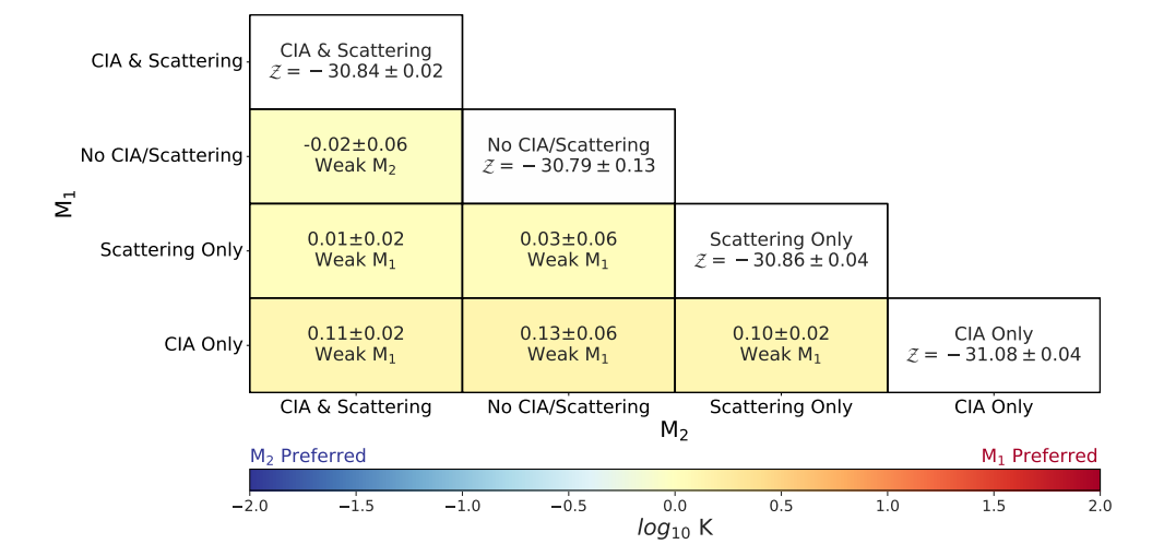
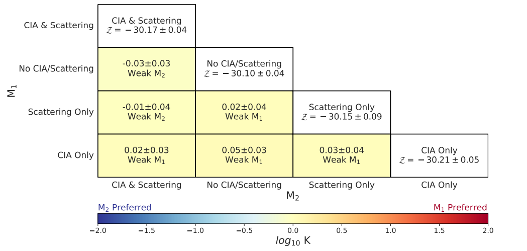
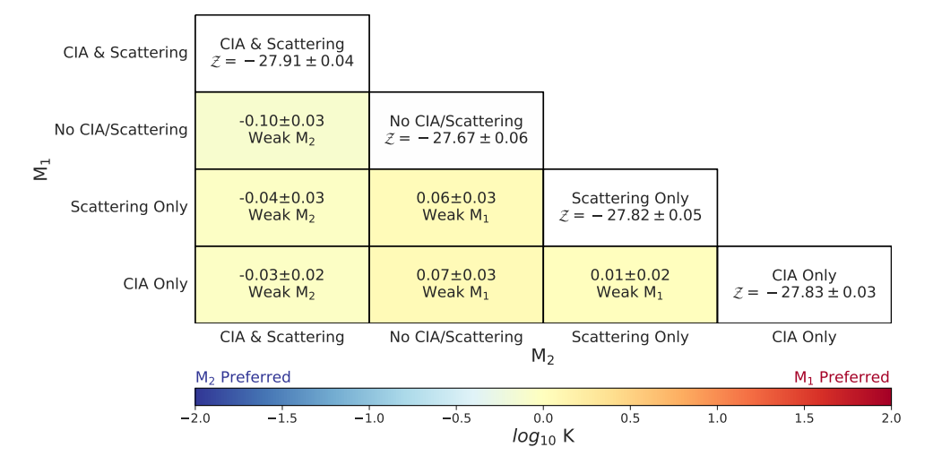
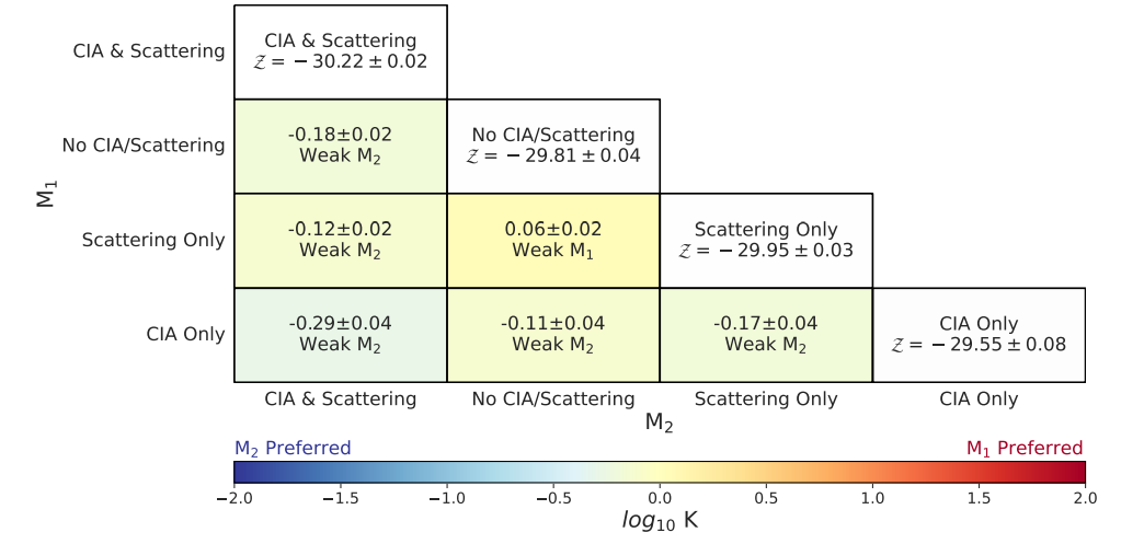
Appendix C: Bayes’ factor analysis: other epochs
Appendix D: Cloudy scenarios: additional figures
Appendix D: Cloudy scenarios: additional figures
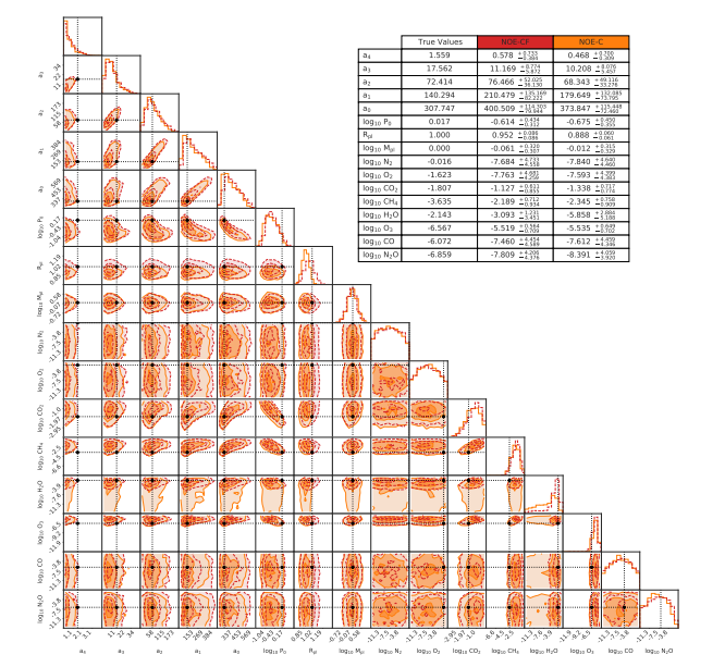
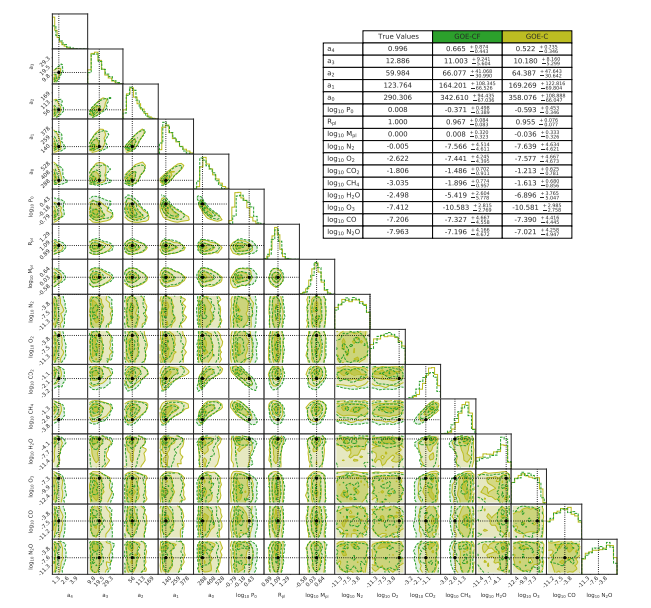
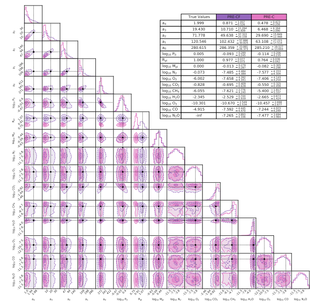
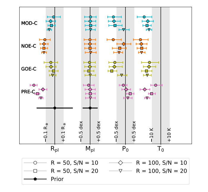
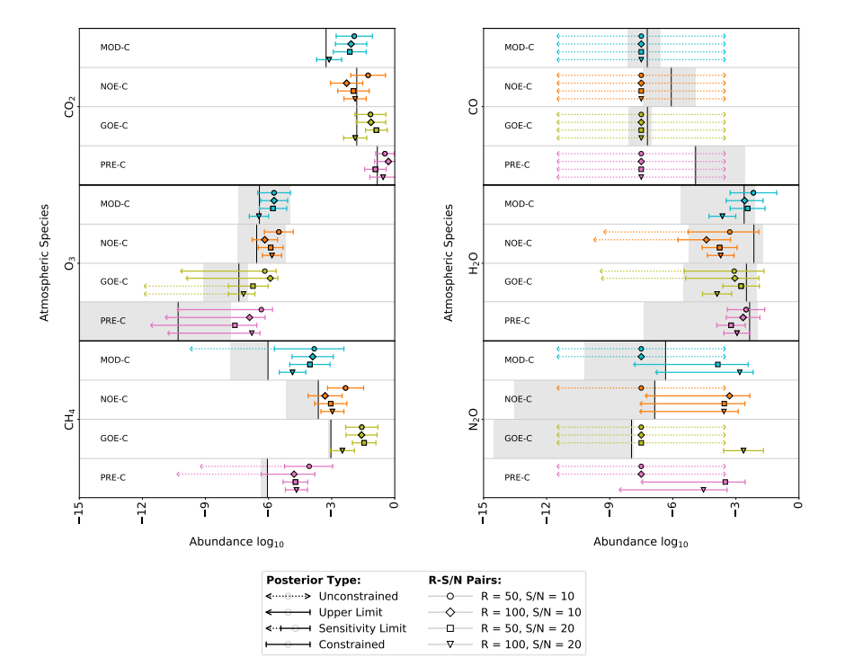
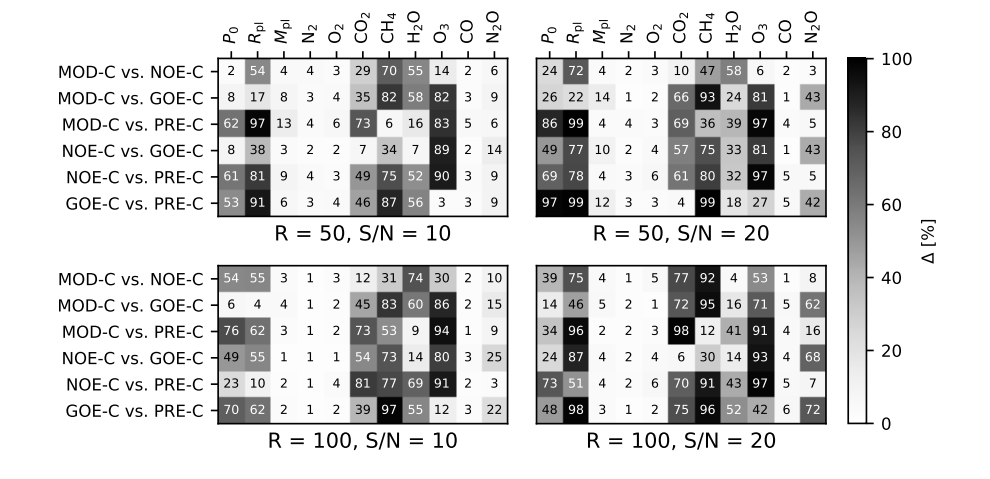
In this section, we provide additional plots for the cloudy scenarios. In Figures D.1 and D.2 we show the retrieved exoplanet parameters and abundances for the different scenarios with varying R and S/N values. Finally, we plot in Figure D.3 the maximum difference ∆ between the cumulative posteriors for the different model parameters, for each combination of the cloudy scenarios and different R-S/N pairs.
This paper is available on arxiv under CC 4.0 license.
[story continues]
tags