The Soup Kitchen Bound: ReLU Inequalities at the Core of Availability vs. Throughput

Table of Links

Abstract and 1. Introduction

2. The Soup Kitchen Problem

   2.1 Model and 2.2 Limits of Throughput and Availability

   2.3 Analysis of Throughput and Availability

3. Multi-Unit Posted-Price Mechanisms

   3.1 Model

   3.2 Results

4. Transaction fee mechanism design

5. Conclusions and future work, and References

A. Proofs for Section 2 (The Soup Kitchen Problem)

B. Proofs for Section 3 (Multi-Unit Posted-Price Mechanisms)

2. The Soup Kitchen Problem

2.1 Model

2.2 Limits of Throughput and Availability

The following high-level sequence of results culminates in our main theorem.

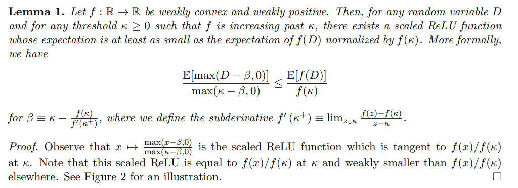
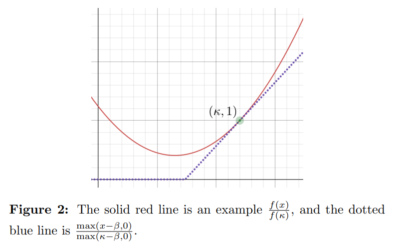
Some functions f in the above theorem will produce stronger bounds, while others will produce weaker bounds. The following lemma can be used to narrow the search space for functions f that produce strong bounds:1

2.3 Analysis of Throughput and Availability

This section sketches the proofs of Theorem 1, Theorem 2, and Theorem 3. Full proofs can be found in the appendix.

One way to conceptualize Theorem 1 is that it demonstrates a set of upper bounds on E[f(D)] that are tight when

To prove Theorem 1, we first show the following lemma:

A proof of Lemma 3 can also be found in other works (Hoeffding, 1956; Arnosti and Ma, 2023), and can be naturally extended to show that E[f(X)] is maximized as the number of demands n → ∞, i.e. as the binomial X approaches a Poisson Y with mean Y] = E[X]. The fact that E[f(X)] ≤ Y)] is used to conclude Theorem 1. Furthermore, observe that E[f(X)] ≤ Y)] additionally implies that the bound in Theorem 3 is weakest when n → ∞.

The proof of Theorem 2 from Theorem 1 is relatively straightforward. It follows a similar structure to Markov’s inequality on the random variable f(D).

Proof of Theorem 2. From the law of total expectation, we have

E[f(D)] = E[f(D) 1(D < κ)] + E[f(D) | D ≥ κ]P(D ≥ κ).

Since f is weakly positive, E[f(D) 1(D < κ)] ≥ 0. Furthermore, since f is weakly convex, E[f(D) | D ≥ κ] ≥ f(E[D | D ≥ κ]). Thus,

f(E[D | D ≥ κ]) P(D ≥ κ) ≤ E[f(D)].

Next, from Theorem 1, we have E[f(D)] ≤ E[f(X)]. Therefore,

f(E[D | D ≥ κ]) P(D ≥ κ) ≤ E[f(X)].

Dividing both sides by f(E[D | D ≥ κ]) ≥ 0, we obtain as desired:

Observe that the most notable difference between Theorem 2 and Markov’s inequality is that the denominator on the right-hand side is f(E[D | D ≥ κ]), not f(κ).

Proving Theorem 3 from Theorem 2 is quite involved.

Proof sketch of Theorem 3. We select the ReLU mapping f(x) = max(x−β, 0) for a value of β ≤ κ, and obtain

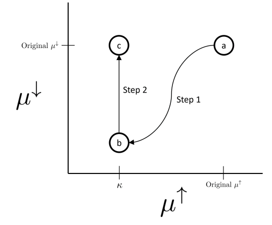
In the case where β < 0, we show directly that the right-hand side is decreasing in µ ↑, and move µ ↑ → κ. In the more complicated case where β ≥ 0, we adjust the parameters of the right-hand side in two steps:

1. Move along a path of pairs (µ↑, µ↓) that keeps the right-hand side constant, and such that the end of the path is the point (κ, t) for some t below the original µ ↓.

2. Adjust t upwards to the original µ↓, and show that this only increases the right-hand side.

Therefore, the final value of the right-hand side should be at least P(D ≥ κ). See Figure 3 for an illustration.

The resulting formula for the right-hand side is equal to the formula for the expectation of a binomial distribution with mean κP(D ≥ κ) + µ ↓ = κτ , divided by the value max(κ − β, 0). A straightforward application of Lemma 1 completes the theorem, showing that this ReLU bound can be weakened to f(X)/f(κ) for X ∼ Binomial(n, κτ /n).

Observe that the ReLU function described in Lemma 1 is weakly convex, weakly positive, and is strictly increasing past κ. It thus satisfies all the requirements for making a concentration inequality using Theorem 3, and we can conclude that for any concentration inequality made using Theorem 3, there exists a ReLU function that produces a concentration inequality at least as strong. This means that in order to find the functions f for use with Theorem 3 that produce the strongest concentration inequalities, it suffices to search solely among the class of ReLU functions.