The Two-Step ML Secret Behind SkyCURTAINs

Table of Links

Abstract and 1. Introduction

2. Dataset

3. SkyCURTAINs Method and 3.1 CurtainsF4F

3.2. Line detection

4. Results

4.1. Metrics

4.2. Full GD-1 stream scan

5. Conclusion, Acknowledgments, Data Availability, and References

APPENDIX A: CurtainsF4F TRAINING AND HYPERPARAMETER TUNING DETAILS

A1. CurtainsF4F features preprocessing

A2. Hyperparameter tuning

3 SkyCURTAINs METHOD

SkyCURTAINs is a two stage approach to find stellar streams in a model agnostic manner. The first stage is CurtainsF4F followed by a CWoLa step. This stage is used to infer a threshold to select the candidate signal stars for the second stage. The first stage flags all overdensities as anomalous. But as we are looking for stellar streams, we need to identify line-like structures in the candidate signal stars’ population. This is done by the second stage of the SkyCURTAINs method, which uses the Hough transform (Hough 1962) for line detection. Details of training and implementation of the two stages are discussed in the following sections.

3.1 CurtainsF4F

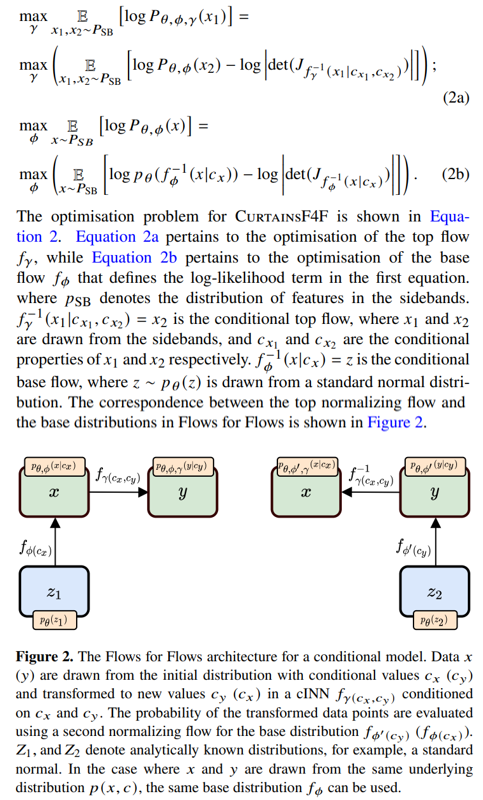
CurtainsF4F constructs a background-enriched template in the signal region by learning a conditional transformation of the features from the sidebands to the signal region, as a function of the proper motion. CurtainsF4F uses a maximum likelihood loss on the transported data and the target data using the Flows for Flows method introduced in Golling et al. (2023) to learn this transformation.

A normalising flow (Papamakarios et al. 2021) is a model that learns a bijective transformation 𝑓𝜙 : 𝑧 → 𝑥 between a base distribution to a target distribution under maximum likelihood, where 𝑧 ∼ 𝑝 𝜃 and 𝑥 ∼ 𝑃𝑋. The usual choice for the base distribution is a standard normal distribution. The loss function for training this normalizing flow 𝑓𝜙 is given by the change of variables formula

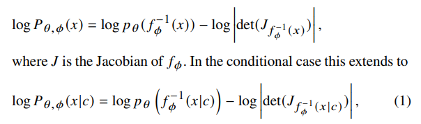
where 𝑐 are the conditional properties, and 𝜙 are the learnable parameters of the normalizing flow 𝑓 , and 𝜃 are the parameters of the base distribution.

In anomaly detection methods such as (Nachman & Shih 2020), one learns the distribution 𝑝𝜙 (𝑥|𝑐) for 𝑐 in the sideband regions, and then queries the conditional normalizing flow for 𝑐 in the signal region to obtain a data-driven model for the background template there. This “automatic" interpolation of the conditional density is simple and effective, however empirically it was found in (Nachman & Shih 2020) that for accurate interpolation into the sideband one needed to train 𝑝𝜙 (𝑥|𝑐) on the entire complement of the signal region. For a sliding window search, it is computationally expensive to train a separate flow on the complement of every signal region. CurtainsF4F improves on this situation by training a second conditional flow to learn a transformation between left and right sideband data. This flow is found to interpolate much better as the transformations to be learnt are much simpler and this simplicity acts as an implicit regularisation when interpolating to the signal region. One can get an accurate background template in the signal region with just training on narrower sidebands instead of the entire complement of the signal region. The procedure of CurtainsF4F also allows one to train a single base flow to learn 𝑝𝜙 (𝑥|𝑐) for the entire data, and then sampling from this in narrow sidebands one can train the top flow to interpolate into any signal region. Thus, the expensive step of training the base flow need only be done once, and then the cheap step of training the top flow can be repeated with much less computational cost.

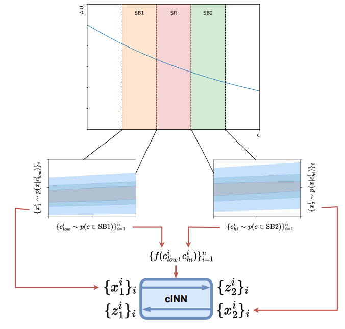
CurtainsF4F is trained in both directions. The forward pass transforms data from low to higher target values of proper motion, whereas the inverse pass transforms data from high to lower target values. Data are drawn from both SBs and target proper motion values are randomly assigned to each data point using all proper motion values in the batch. Data are passed through the network in a forward or inverse pass, depending on whether the proper motion is larger or smaller than their initial proper motion. The network is conditioned on a function of initial and target proper motion, with the two values ordered in ascending order. This function could be, for example, difference between the two, or simply both values concatenated. The probability term is evaluated using a single base distribution trained on the data from SB1 and SB2. The loss for the batch is calculated from the average of the probabilities calculated from the forward and inverse passes. A schematic overview is shown in Figure 3.

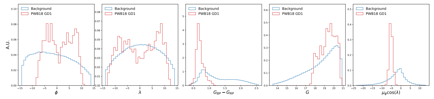
The base flow is trained on the sideband data with a standard normal distribution as the target prior. It is conditioned on the proper motion. The top flow is trained between data drawn from the sidebands. The transformation is conditioned on the concatenated tuple of the initial and target proper motion. Depending on which proper motion is chosen as the conditioning feature, the downstream task of finding the stream might be affected. This is because the stream candidate stars may have a non-trivial correlation, and therefore may produce over densities of different shapes in the two proper motions respectively. In this work, we use 𝜇𝜆 as the conditional feature. The rest of features, i.e. [𝜙, 𝜆, 𝐺, 𝐺BP − 𝐺RP, 𝜇𝜙 cos 𝜆 ] are used to characterise the template.

One important aspect of the CurtainsF4F method is the definition of signal and sideband regions. In Figure 4, we show the distribution of 𝜇𝜆 of the background stars and GD-1 stream stars in the sidebands (SB1, SB2) and signal region (SR). Unlike in the Via Machinae method, where the sideband region was the complementary region of the chosen SR, SkyCURTAINs defines the sideband region to be typically of 2-6 mas/yr. Since the top flow only needs to learn a small (but not necessarily trivial) transformation of the sideband data to generate a template in the SR, we find this width of the sideband to be sufficient. This also cuts down the total training time compared to Via Machinae, as despite both methods consisting of two generative models, SkyCURTAINs’s second generative model effectively learns on narrower sidebands. To demonstrate the efficacy of the method on the GD-1 stream, we define the signal region as the interval in which the signal is contained. In an actual analysis, where the location of the signal is not known a priori, one would need to scan multiple values of 𝜇𝜆 with the CurtainsF4F method. Here, the modularity of the CurtainsF4F method comes into play, as the base flow can be trained on the entire patch of the sky and frozen. Thereafter, top flows can be trained on individual regions of interest. This significantly reduces the computational cost of training the model, by allowing the base flow to be trained once and reused for multiple regions of interest.

Once the CurtainsF4F model is trained, the background-enriched template is constructed by transforming the data from the sidebands to the signal region, conditioned on the tuple of the initial and target proper motion. The target proper motions in the signal region are sampled from a kernel density fit on the proper motion distribution. We train an ensemble of 10 multi-layer perceptron-based classifiers [1]

between this template and the signal region data. The scores are then aggregated by taking the mean score and used to classify the data in the signal region. The top 0.1% most signal-like stars are selected as the candidates for the next step. This threshold is selected to remove the most background like stars from the signal region, which is a tunable parameter and can be adjusted based on the desired purity and signal efficiency.

3.2 Line detection

The CurtainsF4F step gives us a set of stars which produce an over-density in the feature space. We still need to filter out the overdensities that are particularly line like, as we are interested in stellar streams. We employ a well known line finding algorithm to estimate the line parameters of the stream via the Hough transform, as was done in (Shih et al. 2021, 2023). Since we do not apply a fiducial cut to eliminate stars outside a 10◦ radius, we can use the full set of stars that pass the CurtainsF4F cut in the patch to estimate the line parameters.

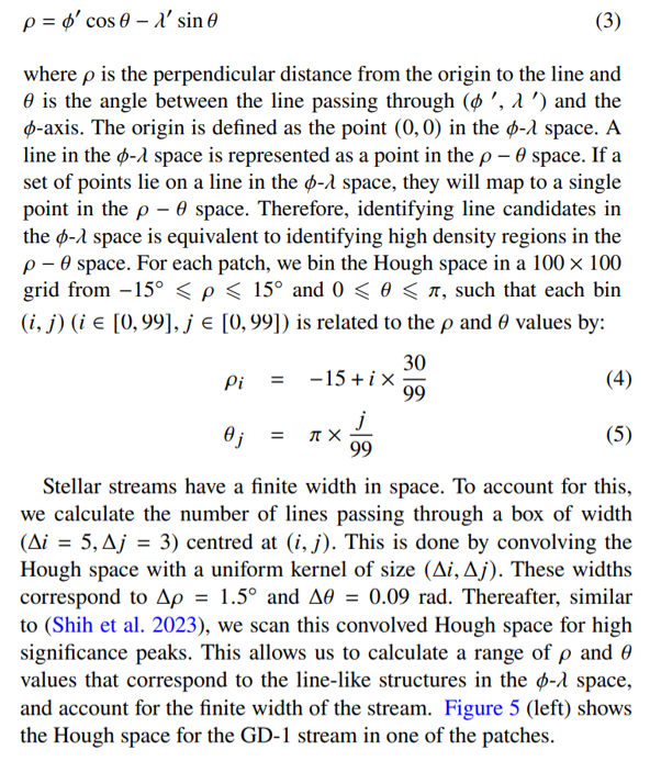
For a given star located at (𝜙′, 𝜆′), the Hough transform is a mapping from the 𝜙-𝜆 space to the parameter space 𝜌 − 𝜃, defined as:

[1] Details about the architecture can be found in Appendix A