Table of Links
-
Hypothesis testing
2.5 Optional Stopping and Peeking
-
Safe Tests
-
Safe Testing Simulations
4.1 Introduction and 4.2 Python Implementation
-
Mixture sequential probability ratio test
5.3 mSPRT and the safe t-test
In this section, we will compare mSPRT and the safe t-test in terms of power, sample size, and other properties.
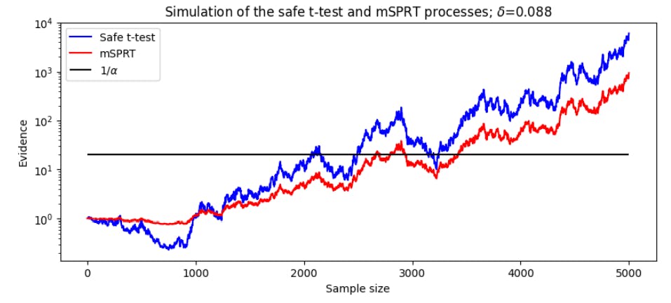
We will first consider the performance of the statistics on a pair of random normal samples with a mean difference of δ and unit variance. Both of the statistics behave as test martingales, so we can compare them visually as they accumulate evidence for and against H0. Figure 8 shows a simulation of these processes.

The first thing to notice is that both tests draw similar conclusions from the data. In the first 1000 samples, there is evidence in favour of H0 : δ = 0 which causes both test statistics to decrease. Following evidence in favour of the alternative hypothesis H1 : δ ̸= 0, both test statistics increase until they cross the 1/α threshold. A second observation is in the magnitude that each test weighs evidence. As evidence initially supports the null hypothesis, the safe test statistic decreases much more quickly than the mSPRT statistic. However, as the data supporting H1 increases, the safe statistic surpasses the mSPRT statistic, staying far above for the remainder of the experiment. A final observation is in when the statistics cross the 1/α threshold. While the safe test needs less than 2100 samples to reject the null, mSPRT needs over 2700 samples.
With an understanding of how the safe t-test and mSPRT perform on a random sample, we can now consider many simulations with the same effect size δ. The goal of these tests is to stop when enough evidence against H0 : δ = 0 has been collected. Therefore, we will compare the 1/α stopping times of these test statistics. In cases for which no effect is detected, the test is stopped at a power of 1 − β = 0.8. Figure 9 shows the result of many simulations of this process.
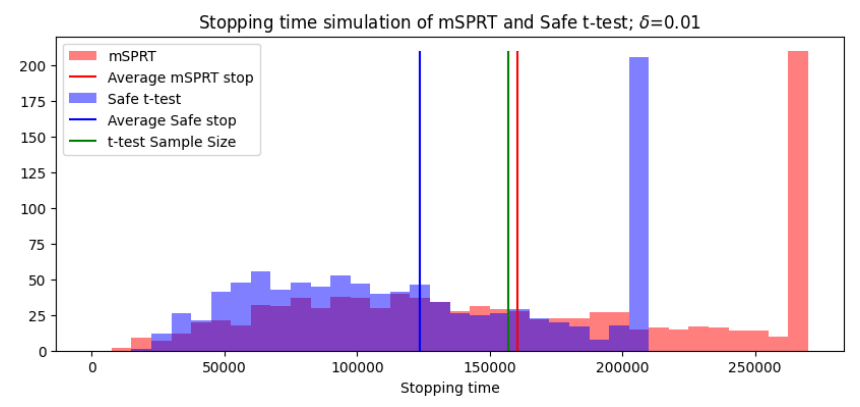
The stopping time histogram in Figure 9 shows that for the simulated data with an effect size of δ = 0.01, safe tests are able to conclude much more quickly than mSPRT. On average, the safe test uses 22% less data than the mSPRT. For tests that do not reach the 1/α threshold, the test is stopped without rejecting the null hypothesis. About 20% of the both the safe test and the mSPRT reach this threshold, as is expected for a test with 80% power. These sample size results can be broken down further based on the result of the test. It is interesting to know, for example, the number of samples required, on average, to reject H0. These results can be seen in Table 2.
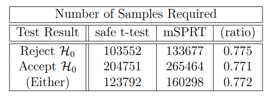
The results of Table 2 are relevant for practitioners who are particularly concerned with deviations from the null hypothesis. Uber, for example, uses mSPRT to monitor outages of their platform [SA23]. Given that the safe t-test rejects H0 with 22% less data, this could decrease the time to recognize outages and hence improve response time.
We’ve seen that for simulations of δ = 0.01 the safe test concludes using fewer samples than the mSPRT, but it remains to be seen for different effect sizes. The following experiment is conducted on 30 effect sizes ranging from 0.01 to 0.3. There are two stopping times we wish to consider: the average stopping time for each test, and the stopping time required for 80% power. To contextualize these results, we can consider the sample size ratio of each of these tests with respect to the classical A/B test. Figure 10 shows the average and maximum stopping times of the safe t-test and the mSPRT, in terms of a sample size ratio of the classical t-test.
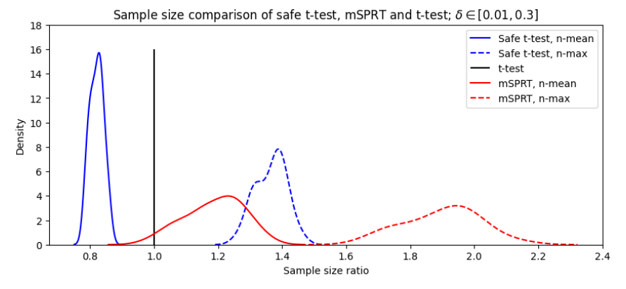
The solid lines in Figure 10 represent the average stopping time of all simulations for all effect sizes. The safe test needs about 20% fewer samples than the t-test, while the mSPRT needs about 20% more. The dashed lines represent the maximum sample sizes required to achieve 1 − β power. While the mSPRT needs about twice as many sample as the t-test to achieve this power, the safe t-test only needs about 40% more samples.
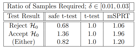
As with Table 2, we can compare the average stopping times for the tests based on whether they reject or accept H0. These results, found in Table 3, show that to reject H0, the safe t-test uses 32% less data than the t-test, while the mSPRT uses 6% more. This provides further evidence that the safe t-test is more efficient than the mSPRT in reaching conclusions with the same data.
To compare the average stopping times as a function of effect size δ, we can again normalize the sample sizes by the classical t-test sample size. The results can be seen in Figure 11.
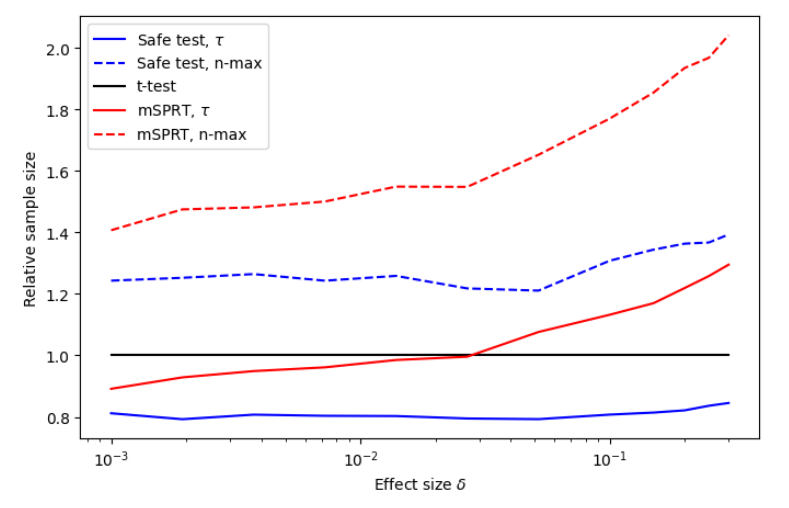
Figure 11 shows that the safe t-statistic sample sizes are smaller than both the classical t-test and the mSPRT for all δ ∈ [0.001, 0.3]. The capability of the safe t-test to detect these small effect sizes is a motivator for the its use in online A/B testing.
Until now, all simulations have been conducted with α = 0.05 and β = 0.2. To assure readers that these parameters are not biasing the results, Figure 12 shows the stopping times when varying these parameters.
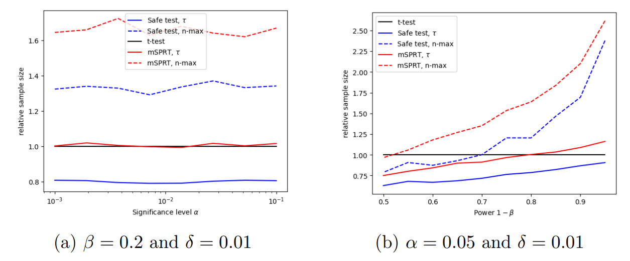
It is clear that the effectiveness of the safe t-test will extend to a variety of testing scenarios based on experimenter’s needs.
In this section, we have compared the safe t-test and the mSPRT through various simulations. It was found that the safe t-test stops earlier than the mSPRT in all simulations. This leads to smaller sample sizes and faster experimentation. We also found that the safe t-test is able to reject H0 with much less data than both the classical t-test and the mSPRT. In the next section, we further analyze the performance of these statistic tests on real A/B test data.
Author:
(1) Daniel Beasley
This paper is
[story continues]
tags