Table of Links
2 Lattice models and coordinate space
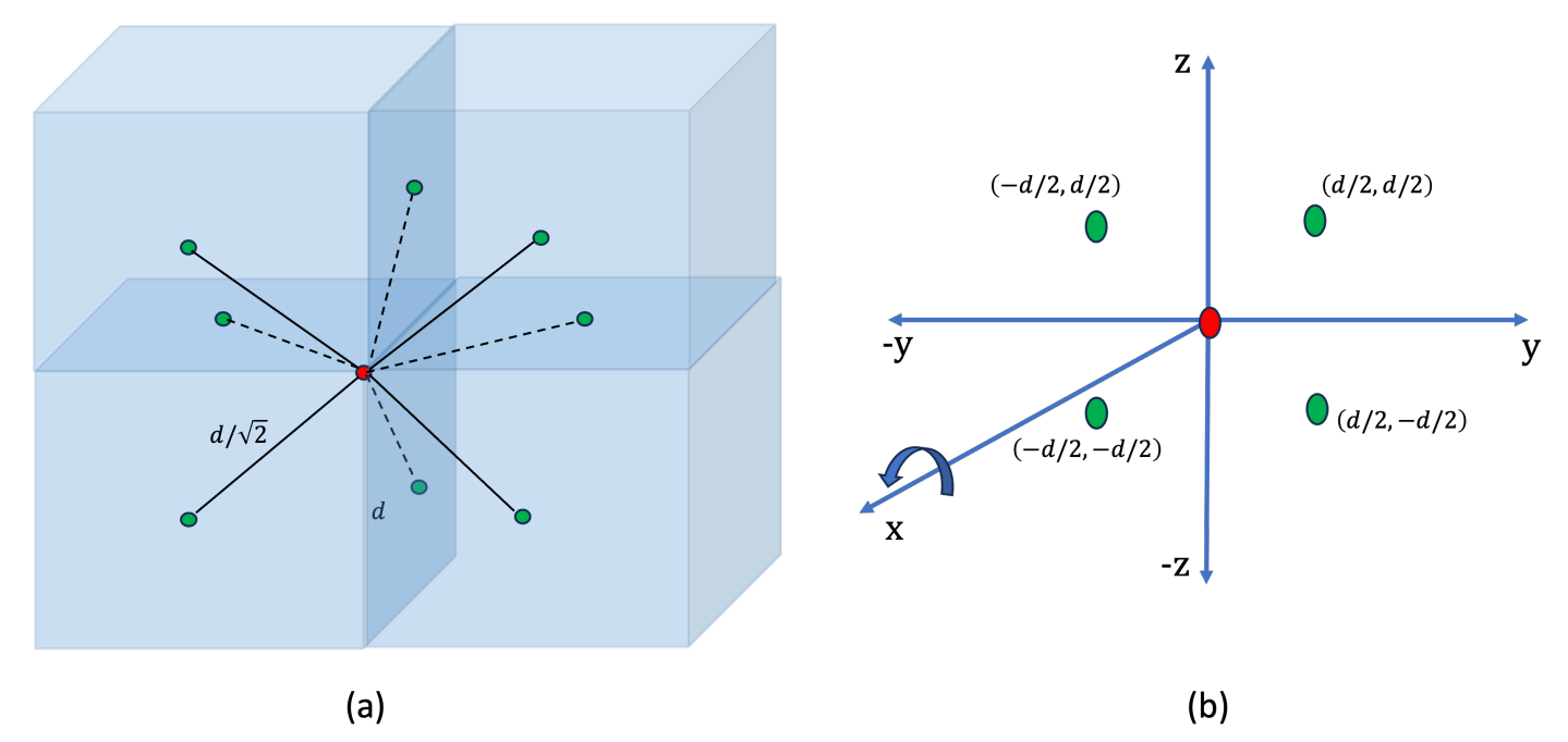
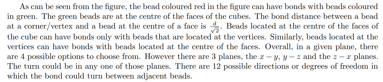
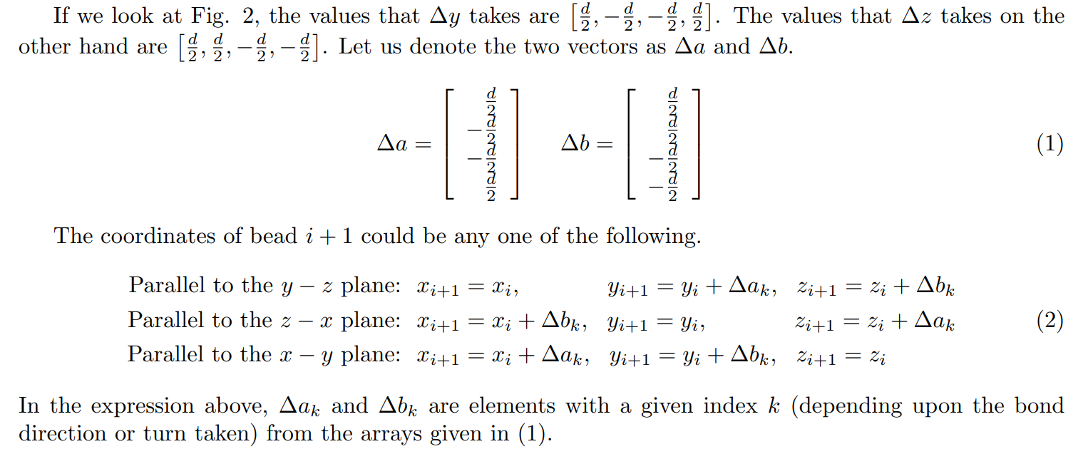
Fig. 2 (a) gives a section of the structure of the FCC lattice. Given a protein bead at the origin, we would like to know the possible set of 3D coordinates that the next bead could take following a turn. Fig. 2 (b) gives the possible coordinates in a given plane y − z.
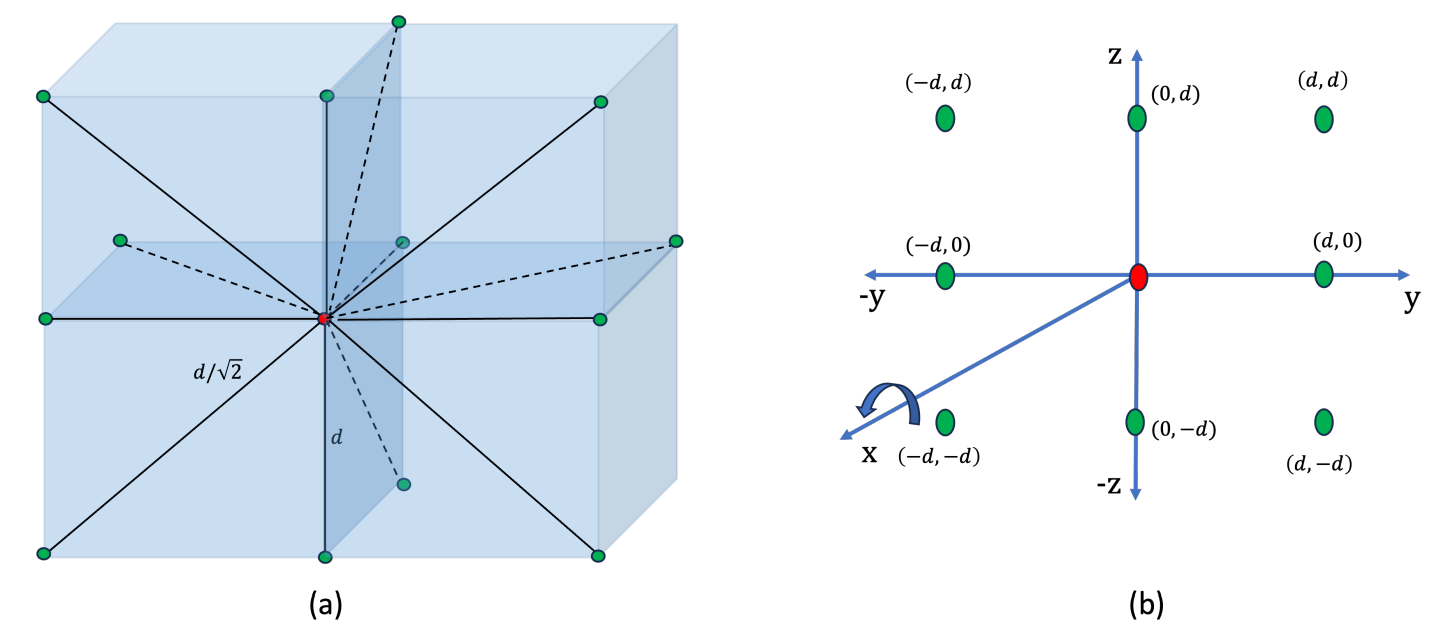
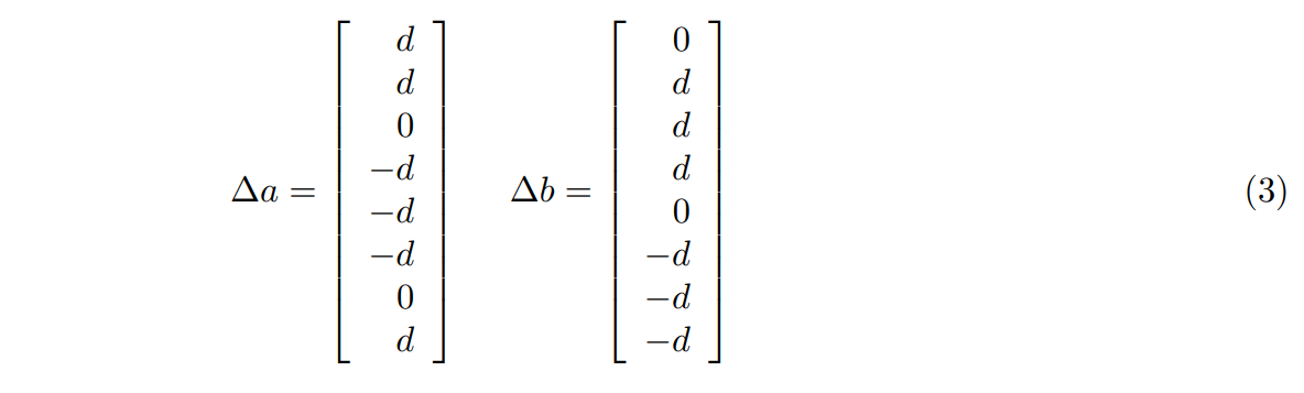
Now, let us have a look at the cubic lattice with planar diagonals. Fig. 3 (a) gives the section of a cubic lattice and 3 (b) gives the coordinate mapping. In the cubic lattice, the turns could be in 8 directions in a given plane. With 3 planes, there are 24 possible turns. However, there for every set of two planes, there are two directions that are repeated. For example, if we consider the x − y plane and the y −z plane, the ±y directions are repeated. As a result, we will have 6 such planes that are repeated. Overall, we will have 24 − 6 = 18 degrees of freedom here.
In order to encode, we need to map the qubit states to bead coordinates. Let us consider the FCC lattice. We can start from the origin as the coordinates of the first bead. The second bead will take up a position at any one of the vertices or faces as shown in Fig. 2 (b). If we denote the axes as x, y and z, the location of the second bead could be in any one of the xy, yz or zx planes. The red bead is at the origin. If the second bead were to be in the y − z plane, the possible coordinates that it could have are shown in the figure. The coordinates are the y and z coordinates given as (y, z). This is a rotation around the x-axis at 90◦ interval for 4 different points, in a counter-clockwise direction. We would see a similar set of coordinates in the z − x and x − y plane if the second bead were to be in the those planes. In Fig. 2 (b) the x coordinates of the red and green beads are the same. We could carry forward this logic to every bead in the protein sequence. If we consider any bead i with coordinates (x, y, z), the bead i + 1 would then have coordinates (x + ∆x, y + ∆y, z + ∆z). If the bead i + 1 is in the plane parallel to the y − z plane, ∆x = 0 and ∆y and ∆z would take values as shown in Fig. 2 (b). If it is in the plane parallel to the z − x plane (counter-clockwise rotation around y-axis), ∆z and ∆x would take up the same values as ∆y and ∆z in the previous case, and in the same order. Similarly, when the the bead i + 1 is in the plane parallel to the x − y plane (counter-clockwise rotation around z-axis), ∆x and ∆y would take up similar values.
Similarly, with the cubic lattice with planar diagonals, there are 8 possible directions. The vectors ∆a and ∆b will have the form shown in (3).
3 Encoding to qubit states
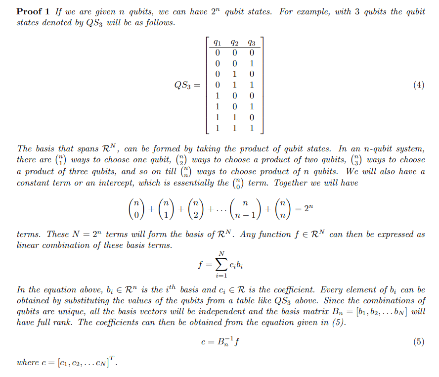
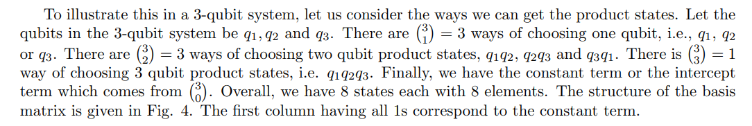
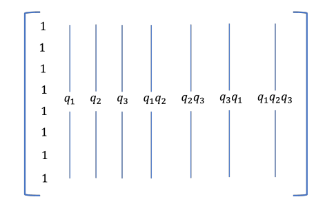
3. 3.1 Encoding lattice structure in qubit sta
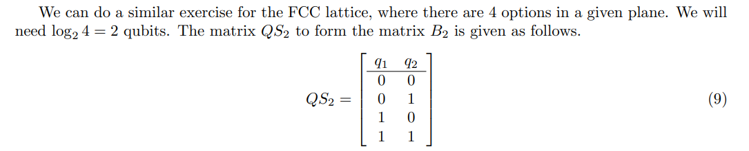
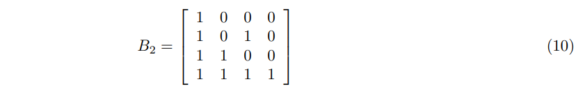
The basis B2 will have the form shown in Fig. 5. By substituting the values of the q1 and q2 in QS2 in
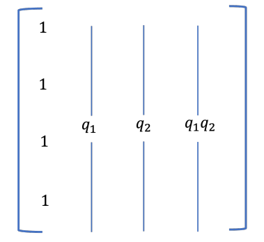
the matrix given in Fig. 5, we will get the basis matrix B2 as given below.
As in the previous case, the vectors ∆a and ∆b in (1) can be represented using the basis vectors in B2. The coefficients can be estimated the following way.

The coefficients obtained for the FCC lattice are as follows.
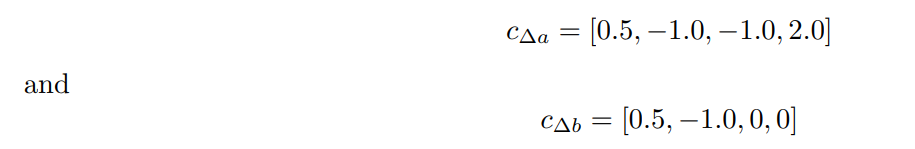
We can thus express ∆a and ∆b as follows.

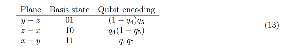
3.2 Selection of the plane of turn
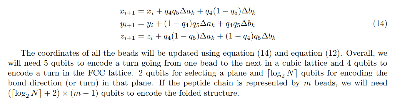
Since there are 3 orthogonal planes (x − y, y − x and z − x), we need two more qubits more to make a selection of one of the planes. Let these two qubits be denoted as q4 and q5. The selection could be based on the computational basis states of the q4 and q5 as follows.
With the given selection criteria, we have to update equation (2) as follows.
3.3 Extending it to other structures
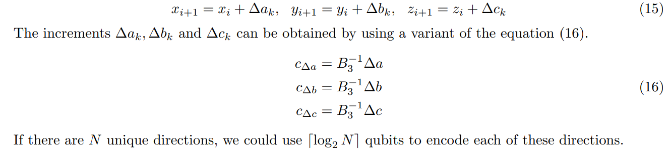
This concept can be extended to other lattice structures as well. We need not have turns along orthogonal planes like the cubic or FCC lattices. The planes could be at an angle to the working plane. As long as the every bead or lattice point has equal and identical degrees of freedom, we could use the methodology explained here. In case, the lattice involves directions that are always at angle, we could do away with the qubits involved in plane selection and directly go for encoding directions to the computational basis states. Under such circumstances, the coordinate updates following a turn would be of the form given in (15).
4 Conclusions
In this article, we discussed a methodology to encode lattice turns to qubit computational basis states, that could find use in protein structure prediction, polymer structure study and other coarse-grained models. We showed how a combination of qubit states could be used to span the space of directions. These directions could be along planes that are orthogonal or non-orthogonal to each other. We took specific examples of cubic and FCC lattice. However, they could be extended to other lattice structures as well.
References
[1] W. E. Hart and A. Newman, “Protein structure prediction with lattice models,” http://dimacs. rutgers.edu/∼alantha/papers2/alantha-bill-bc.pdf.
[2] S. Kmiecik and et. al., “Coarse-grained protein models and their applications,” ACS Chem. Rev., vol. 116, pp. 7898–7936, June 2016.
[3] M. Fingerhuth, T. Babej, and C. Ing, “A quantum alternating operator ansatz with hard and soft constraints for lattice protein folding,” arXiv preprint arXiv:1810.13411, 2018.
[4] A. Perdomo, C. Truncik, I. Tubert-Brohman, G. Rose, and A. Aspuru-Guzik, “Construction of model hamiltonians for adiabatic quantum computation and its application to finding low-energy conformations of lattice protein models,” Phys. Rev. A, vol. 78, p. 012320, Jul 2008.
[5] A. Robert, P. Barkoutsos, S. Woerner, and I. Tavernelli, “Resource-efficient quantum algorithm for protein folding,” npj Quantum Information, vol. 7:38, 2021.
[6] J. P. Vasavi and et. al., “An approach to solve the coarse-grained protein folding problem in a quantum computer,” arXiv preprint arXiv:2311.14141v1, 2023.
Author:
(1) Kalyan Dasgupta, IBM Research, Bangalore, India.
This paper is
[story continues]
tags