Authors:
(1) David Binder, University of Tübingen, Germany;
(2) Marco Tzschentke, University of Tübingen, Germany;
(3) Marius Muller, University of Tübingen, Germany;
(4) Klaus Ostermann, University of Tübingen, Germany.
Table of Links
-
Translating To Sequent Calculus
-
Evaluation Within a Context
-
Insights
5.1 Evaluation Contexts are First Class
5.3 Let-Bindings are Dual to Control Operators
5.4 The Case-of-Case Transformation
5.5 Direct and Indirect Consumers
-
Conclusion, Data Availability Statement, and Acknowledgments
A. The Relationship to the Sequent Calculus
C. Operational Semantics of label/goto
1 Introduction
Suppose you have just implemented your own small functional language. To test it, you write the following function which multiplies all the numbers contained in a list:
def mult(𝑙) ≔ case 𝑙 of { Nil ⇒ 1, Cons(𝑥, 𝑥𝑠) ⇒ 𝑥 ∗ mult(𝑥𝑠) }
What bugs you about this implementation is that you know an obvious optimization: The function should directly return zero if it encounters a zero in the list. There are many ways to achieve this, but you choose to extend your language with labeled expressions and a goto instruction. This allows you to write the optimized version:
def mult(𝑙) ≔ label 𝛼 { mult’(𝑙; 𝛼) }
def mult’(𝑙; 𝛼) ≔ case 𝑙 of { Nil ⇒ 1, Cons(𝑥, 𝑥𝑠) ⇒ ifz(𝑥, goto(0; 𝛼), 𝑥 ∗ mult’(𝑥𝑠; 𝛼)) }
Here is how you read this snippet: Besides the list argument 𝑙, the definition def mult(𝑙; 𝛼) ≔ . . . takes an argument 𝛼 which indicates how the computation should continue once the result of the multiplication is computed (we again use ; to separate these two kinds of arguments). The helper function mult’ takes a list argument 𝑙 and two arguments 𝛼 and 𝛽; the argument 𝛽 indicates where the function should return to on a normal recursive call while 𝛼 indicates the return point of a short-circuiting computation. In the body of mult’ we use ⟨𝑙 | case {Nil ⇒ . . . , Cons(𝑥, 𝑥𝑠) ⇒ . . .}⟩ to perform a case split on the list 𝑙. If the list is Nil, then we use ⟨1 | 𝛽⟩ to return 1 to 𝛽, which is the return for a normal recursive call. If the list has the form Cons(𝑥, 𝑥𝑠) and 𝑥 is zero, we return with ⟨0 | 𝛼⟩, where 𝛼 is the return point which short-circuits the computation. If 𝑥 isn’t zero, then we have to perform the recursive call mult’(𝑥𝑠; 𝛼, 𝜇𝑧. ˜ ∗ (𝑥, 𝑧; 𝛽)), where we use 𝜇𝑧. ˜ ∗ (𝑥, 𝑧; 𝛽) to bind the result of the recursive call to the variable 𝑧 before multiplying it with 𝑥 and returning to 𝛽. Don’t be discouraged if this looks complicated at the moment; the main part of this paper will cover everything in much more detail.
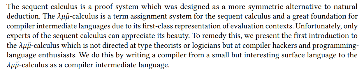
The 𝜆𝜇𝜇˜-calculus that you have just seen was first introduced by Curien and Herbelin [2000] as a solution to a longstanding open question: What should a term language for the sequent calculus look like? The sequent calculus is one of two influential proof calculi introduced by Gentzen [1935a,b] in a single paper, the other calculus being natural deduction. The term language for natural deduction is the ordinary lambda calculus, but it was difficult to find a good term language for the sequent calculus. After it had been found, the 𝜆𝜇𝜇˜-calculus was proposed as a better foundation for compiler intermediate languages, for example by Downen et al. [2016]. Despite this, most language designers and compiler writers are still unfamiliar with it. This is the situation that we hope to remedy with this pearl.
We frequently discuss ideas which involve the 𝜆𝜇𝜇˜-calculus with students and colleagues and therefore have to introduce them to its central ideas. But we usually cannot motivate the 𝜆𝜇𝜇˜-calculus as a term assignment system for the sequent calculus, since most of them are not familiar with it. We instead explain the 𝜆𝜇𝜇˜-calculus on the whiteboard by compiling small functional programs into it. Such an introduction is regrettably still missing in the published literature; most existing presentations either presuppose knowledge of the sequent calculus or otherwise spend a lot of space introducing it first. We believe that if one can understand the lambda calculus without first learning about natural deduction proofs, then one should also be able to understand the 𝜆𝜇𝜇˜-calculus without knowing the sequent calculus[1].
Why are we excited about the 𝜆𝜇𝜇˜-calculus, and why do we think that more people should become familiar with its central ideas and concepts? The main feature which distinguishes the 𝜆𝜇𝜇˜- calculus from the lambda calculus is its first-class treatment of evaluation contexts. An evaluation context is the remainder of the program which runs after the current subexpression we are focused on finishes evaluating.
This becomes clearer with an example: When we want to evaluate the expression (2 + 3) ∗ 5, we first have to focus on the subexpression 2 + 3 and evaluate it to its result 5. The remainder of the program, which will run after we have finished the evaluation, can be represented with the evaluation context □ ∗ 5. We cannot bind an evaluation context like □ ∗ 5 to a variable in the lambda calculus, but in the 𝜆𝜇𝜇˜-calculus we can bind such evaluation contexts to covariables. Furthermore, the 𝜇-operator gives direct access to the evaluation context in which the expression is currently evaluated. Having such direct access to the evaluation context is not always necessary for a programmer who wants to write an application, but it is often important for compiler implementors who write optimizations to make programs run faster. One solution that compiler writers use to represent evaluation contexts in the lambda calculus is called continuation-passing style. In continuation-passing style, an evaluation context like □∗5 is represented as a function 𝜆𝑥.𝑥 ∗5. This solution works, but the resulting types which are used to type a program in this style are arguably hard to understand. Being able to easily inspect these types can be very valuable, especially for intermediate representations, where terms tend to look complex. The promise of the 𝜆𝜇𝜇˜-calculus is to provide the expressive power of programs in continuation-passing style without having to deal with the type-acrobatics that are usually associated with it.
The remainder of this paper is structured as follows:
• In Section 2 we introduce the surface language Fun and show how we can translate it into the sequent-calculus-based language Core. The surface language is mostly an expression-oriented functional programming language, but we have added some features such as codata types and control operators whose translations provide important insights into how the 𝜆𝜇𝜇˜-calculus works. In this section, we also compare how redexes are evaluated in both languages.
• In Section 3 we discuss static and dynamic focusing, which are two closely related techniques for lifting subexpressions which are not values into a position where they can be evaluated.
• Section 4 introduces the typing rules for Fun and Core and proves standard results about typing and evaluation.
• We show why we are excited about the 𝜆𝜇𝜇˜-calculus in Section 5. We present various programming language concepts which become much clearer when we present them in the 𝜆𝜇𝜇˜-calculus: We show that let-bindings are precisely dual to control operators, that data and codata types are two perfectly dual ways of specifying types, and that the case-of-case transformation is nothing more than a 𝜇-reduction. These insights are not novel for someone familiar with the 𝜆𝜇𝜇˜-calculus, but not yet as widely known as they should be.
• Finally, in Section 6 we discuss related work and provide pointers for further reading. We conclude in Section 7.
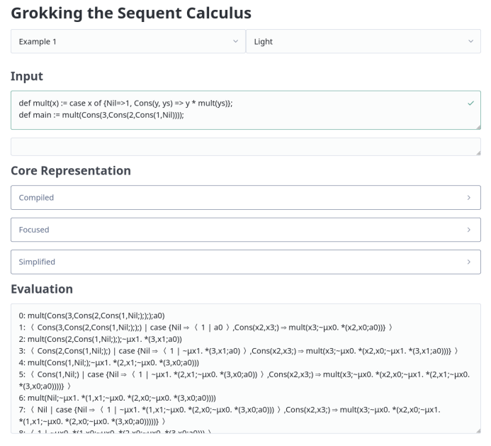
This paper is accompanied by a Haskell implementation which we also make available as an interactive website (cf. Figure 1). You can run the examples presented in this paper in the online evaluator.
This paper is
[1] For the interested reader, we show in Appendix A how the sequent calculus and the 𝜆𝜇𝜇˜-calculus are connected.
[story continues]
tags