Say we are training an LLM or any other DL model. Sometimes we just have this feeling that training is too slow. We didn’t pay for our GPUs to sit idle. We want to use them as efficiently as possible. How can we speed things up? What is the best performance we can aim for?
Properly benchmarking code is a challenge of its own. In one of theprevious articles, we’ve discussed how to do this correctly and what pitfalls are hidden in benchmarking: CPU overhead, L2 cache, etc. Go check that post out if you haven't already! But let’s imagine we have a properly set-up benchmark which shows that the matmul kernel takes 1ms. Is this bad or good? Today, we’re going to learn how to answer these kinds of questions and understand how far we are from hitting the hardware limits.
Three pillars of any GPU code
There are three main components that contribute to the overall kernel time:
- Memory access time. For example, reading an input tensor from (or writing to) large and slow HBM has its cost.
- Compute time. For instance, matrix multiplication primarily relies on Tensor Cores, and they have their own hardware limits, capping the gemm performance depending on the GPU generation.
- Overhead. Any overhead, really. Kernel scheduling is not free, it takes ~10 microseconds to launch even the smallest kernel, and there’s also the CPU overhead that appears when the GPU kernel is “smaller” than the CPU work associated with its launch.
Good news: memory and compute are pretty easy to estimate. While overhead can dominate short benchmarks or micro-kernels, across all training steps it is usually amortized, and for our roofline-style reasoning we can focus on memory and compute without leaving anything interesting on the table.
GPU model
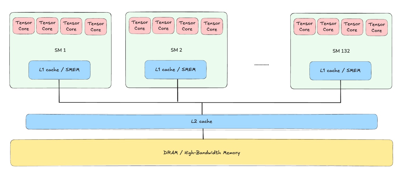
Any modern GPU is a collection of compute cores that are connected to a memory unit. For the purpose of this article, let’s focus on H100 SXM.
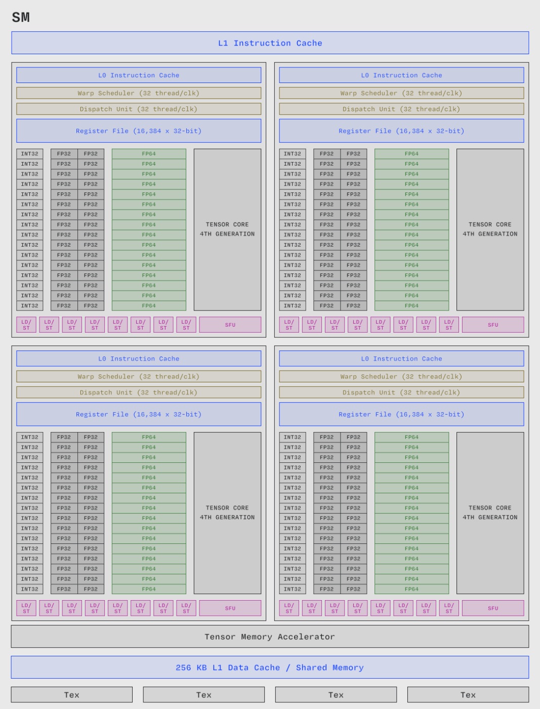
Compute cores are called Streaming Multiprocessors (SMs), and a single H100 has 132 of them. Each SM consists of 4 identical parts, called SM subpartitions. Each subpartition has a single Tensor Core (a dedicated matrix multiplication core), CUDA cores that do arithmetic operations, and 16k 32-bit registers (the local memory). Essentially, each SM is capable of executing instructions in parallel with other SMs. There are more complicated parts, but they are out of the scope of this article.
Each GPU is capable of running a specific number of FLOPs (floating point operations) per second, and thanks to Tensor Cores the number of FLOPs we can utilize is extremely high. Usually the number of FLOPs/s heavily depends on the data type we’re using: when multiplying FP8 matrices we can get twice as many FLOPs/s as when multiplying in BF16. For instance, on H100 the theoretical peak throughput is around 990 TFLOPs/s for BF16, where TFLOPs means tera = 10^12.
There’s also a memory hierarchy associated with a GPU. Specifically, the largest chunk of memory is called HBM (high-bandwidth memory), and when we hear that “H100 has 80GB of memory”, it’s the HBM size we are talking about. There are also L2 and L1 caches, which are both faster and smaller than HBM, that help reduce the memory load when delivering data from HBM to local memory of each SM - registers.
To run any computation on tensors - either model weights, gradients, intermediate activations, etc. - we have to “deliver” them from HBM where they normally reside into the SMs, so the bottleneck is usually the HBM transfer speed. Looking at the H100 specifications, we can see that the HBM has a memory bandwidth (the delivery speed from HBM to tensor cores) of approximately 3.3TB/s. In practice, however, I usually multiply this by 0.7-0.8, which gives us ~2.4TB/s.
Estimating memory
Now, knowing how the GPU memory works, we can estimate the time it takes for our kernel to process everything memory-transfer-related.
If we need to transfer N bytes to or from HBM, we can use 2.4 TB/s for the roofline analysis, and just divide the number of bytes by the memory bandwidth. Usually, we have to read the input and write the result, so we have to sum these two times. Let’s take a look at some examples.
Adding two matrices
Imagine we want to add two FP32 matrices, each of shape 2048 by 4096ю
fp32[2048, 4096] + fp32[2048, 4096] gives us 2 reads and 1 write, all of the same shape, each having 2048*4096*4 bytes (4 bytes per element for FP32).
This gives us a theoretical lower bound of 2048*4096*4 * (2 + 1) / 3.3e12 * 1000 ~ 0.03ms
import torch
import triton


def kernel(a, b):
   c = a + b
   return c


def get_data():
   a = torch.randn((2048, 4096), dtype=torch.float32, device="cuda")
   b = torch.randn((2048, 4096), dtype=torch.float32, device="cuda")
   return a, b

a, b = get_data()
triton.testing.do_bench(lambda: kernel(a, b))  # 0.04ms
This numbers show that our theoretical lower bound is 75% from what we got in real benchmark, so we will be using 2.4 TB/s for future calculations.
Multiply two matrices
Let’s consider only the memory transfers.
To multiply fp32[2048, 4096] @ fp32[4096, 2048], we have to issue two reads of 2048*4096*4 bytes and then issue one write of 2048*2048*4 bytes. In total we get (2048*4096*4*2 + 2048*2048*4)/2.4e12 ~ 0.035ms - even less than for addition. However, there’s also a compute cost that we don’t yet know how to account for.
Estimating compute
We can calculate the number of floating-point operations our kernel performs, and divide it by the max reported FLOPs/s for the specific GPU model. In practice, however, we still want to use 80% of the reported value. Also, if we take a look at the official NVIDIA website, it reports 2x the FLOPs/s we should actually use - that’s because they report FLOPs/s assuming sparsity, which we never achieve in practice. All of these considerations suggest that we should use 800 TFLOPs/s for BF16 compute on H100 instead of 1980 (1980 sparse → 990 no sparsity → 800 practical).
Multiply two matrices
To multiply two matrices of shapes (n, m) and (m, k), we need n * k * 2m operations. The resulting matrix has shape n by k, and each element is the result of a dot product of two m-sized vectors (m multiplications + m-1 additions ~ 2m operations per output element).
For bf16[2048, 4096] @ bf16[4096, 2048], we need 2048 * 4096 * 2048 * 2 / 800e12 ~ 0.043ms.
import torch
import triton


def kernel(a, b):
    c = a @ b
    return c


def get_matrices():
    a = torch.randn((2048, 4096), dtype=torch.bfloat16, device="cuda")
    b = torch.randn((4096, 2048), dtype=torch.bfloat16, device="cuda")
    return a, b


a, b = get_matrices()
triton.testing.do_bench(lambda: kernel(a, b))  # 0.0486533882809274ms
In practice, we get 0.048ms, showing us that the matrix multiplication is a heavily optimized operation.
Theoretical exercises
A few quick sanity checks help build intuition here.
GEMV - Multiplying a vector by a matrix
Say we want to multiply a bf16 vector of size 8192 by a bf16 matrix of shape 8192, 4096. We need 4096*8192*2 FLOPs, so the runtime should be 4096*8192*2/800e12 ~ 0.08 microseconds. However, we need to transfer (8192 + 8192*4096 + 4096)*2 bytes, giving us a memory time of (8192 + 8192*4096 + 4096)*2 / 2.4e12 ~ 0.028ms. As expected, the memory time dominates the compute time, so the kernel is memory-bound, and its runtime is approximately 0.03ms.
a = torch.randn((8192), dtype=torch.bfloat16, device="cuda")
b = torch.randn((8192, 4096), dtype=torch.bfloat16, device="cuda")

triton.testing.do_bench(lambda: a @ b)  # 0.03761992079325684, close to our estimate
As a side note, this is one way to think about why prefill and decode behave so differently: prefill uses compute-bound GEMMs, because it needs to process the full prompt, and decoding usually uses 1-4 tokens, so becomes memory-bound GEMV.
Why we need Flash Attention
Let’s roughly estimate the runtime of a naive Grouped Query Attention forward pass. We’ll use non-causal attention for simplicity. I will skip .transpose and .reshape calls for clarity.
import torch
from einops import einsum

nh = 64  # number of q-heads
nkvh = 4  # number of kv-heads

seqlen = 4096
# nh, nkvh and head_dim follow the Qwen-235B config:
# https://huggingface.co/Qwen/Qwen3-235B-A22B/blob/main/config.json
head_dim = 128

# using (nkvh, ngroups) layout for simplicity
q = torch.randn((nkvh, nh // nkvh, seqlen, head_dim), dtype=torch.bfloat16, device="cuda")
k = torch.randn((nkvh, head_dim, seqlen), dtype=torch.bfloat16, device="cuda")
v = torch.randn((nkvh, seqlen, head_dim), dtype=torch.bfloat16, device="cuda")

def naive_attention():
    qk = einsum(
        q, k, "nkvh ng seqlen_q hd, nkvh hd seqlen_kv -> nkvh ng seqlen_q seqlen_kv"
    )
    qk = qk / head_dim**0.5
    # calculate softmax in FP32, then cast back to BF16
    scores = torch.softmax(qk.float(), dim=-1).to(qk.dtype)
    return einsum(
        scores,
        v,
        "nkvh ng seqlen_q seqlen_kv, nkvh seqlen_kv hd -> nkvh ng seqlen_q hd",
    )
There are the following operations:
QK computation
- Load Q from HBM
- Load K
- Store QK to HBM
Normalization
- Load QK to normalize, store normalized QK
- Load normalized QK in BF16 and store it in FP32 (for softmax upcasting)
Softmax
- Load normalized QK in FP32 inside of a softmax (possibly twice, including the load for
max, but we count it as one) - Store softmax in FP32
- Load softmax in FP32 and store softmax in BF16
Out projection
- Load softmax in BF16
- Load V
- Store O
estimate = (
    (
        nh * seqlen * head_dim * 2  # load q in bf16
        + nkvh * seqlen * head_dim * 2  # load k in bf16
        + nh * seqlen * seqlen * 2 * 3  # store qk, load qk, store qk/sqrt - all in bf16
        + nh * seqlen * seqlen * 4 * (0.5 + 1) # load in bf16, store in fp32
        + nh * seqlen * seqlen * 4 * (2 + 1 + 0.5) # load&store in fp32, load in fp32 to cast to bf16
        + nh * seqlen * seqlen * 2  # load softmax in bf16
        + nkvh * seqlen * head_dim * 2  # load v in bf16
        + nh * seqlen * head_dim * 2  # store o in bf16
    )
    / 2.4e12  # memory bandwidth estimate
    * 1000  # to get ms
)

real, estimate  # 11.79ms, 12.58ms
Now, if we were to estimate the computational time, we’d get:
estimate = (
    2 * nh * seqlen * seqlen * head_dim  # q @ k
    + 2 * nh * seqlen * head_dim * seqlen  # scores @ v
) / 800e12 * 1000  # 0.68
The naive attention implementation is therefore severely memory-bound (compute-time << memory-time).
Flash Attention (https://arxiv.org/pdf/2205.14135, https://arxiv.org/pdf/2307.08691, https://arxiv.org/abs/2407.08608) addresses this issue by fusing all operations in SRAM without materializing intermediate tensors to HBM.
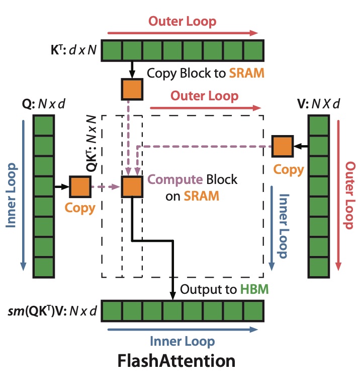
With Flash Attention, the memory traffic is estimated as:
estimate = (
    (
        nh * seqlen * head_dim * 2  # load q in bf16
        + nkvh * seqlen * head_dim * 2  # load k in bf16
        + nkvh * seqlen * head_dim * 2  # load v in bf16
        + nh * seqlen * head_dim * 2  # store o in bf16
    )
    / 2.4e12  # memory bandwidth estimate
    * 1000  # to get ms
)

estimate  # 0.06
In practice, Flash Attention also writes additional meta-information, such as lse (logsumexp), but we’d neglect this for simplicity. Flash attention makes attention compute-bound (there’re always some considerations, though: for example, the very small batch sizes might make us memory-bound again).
This is a good example of roofline estimations becoming a centerpiece for decision-making and optimization.
Small practical examples
torch.zeros() vs. torch.empty()
Say we want to allocate an output buffer for some operation, for example, to write the results of deep_gemm, quantization, all_gather, or anything that requires a pre-allocated buffer. A common practice is to allocate this buffer with torch.zeros() even if we don’t actually need exact zeros there, and even if the values will be overwritten anyway. In fact, torch.zeros() calls torch.empty() followed by a kernel to fill the tensor with zeros! And we can estimate the runtime of this kernel now: it takes (tensor size) / (memory bandwidth).
Imagine that we’re running FP8 dequantization and want to allocate a BF16 buffer for MoE expert weights. This wastes num_experts * hidden * intermediate * 2 / 2.4e12 ~ 0.67ms (for Qwen-235B). If this happens on every layer, for a 64-layer network we waste 42ms just to allocate an unnecessary buffer! For models of this sort, the end-to-end training iteration rarely exceeds 10 seconds at scale, so 0.5% of the iteration time is wasted filling tensors with zeros.
nan_to_num vs zero_()
Imagine you need to choose: allocate a new tensor with .zero_() or use .empty(), but if you use empty, some elements might become NaN, and you’d need to convert them to zeros with .nan_to_num(). Which one is better? Well, we know that zeroing is expensive, and obviously zeroing only some elements is cheaper than zeroing out the full tensor. Right? Unfortunately, the harsh truth is that .zero_() is twice as fast. To zero out a tensor, you only need to write, and no reads are required. For .nan_to_num, you also have to know whether an element is nan or not, so you must read the full tensor and also write it back with updated values. So .nan_to_num is always slower.
MoE grouped gemm 💔 Tensor Parallel
Say we have a SwiGLU MLP inside an MoE block - just three matrices of specific shapes that participate in a few GEMM operations. For instance, our two matrices have shapes (num_experts, hidden, intermediate) and (mbs * seqlen * topk, hidden), where mbsis the micro-batch size.
Let’s consider two different parallelism strategies: tensor parallel and expert parallel. In TP, the intermediate dim is split across TP gpus (TP chunks), and the num_experts-axis will remain intact. In EP, the situation is reversed: the 0-axis is split on EP equal chunks, and the intermediate dim stays the same.
from matplotlib import pyplot as plt
import numpy as np
import pandas as pd
import seaborn as sns
from matplotlib.ticker import FuncFormatter


sns.set_style("whitegrid")
sns.set_context("notebook", font_scale=1.0)

sizes = [2, 4, 8, 16, 32, 64]
top_k = 8
experts = 256
n = 8192
m = 4096
k = 1536

ep, tp = 1, 1
points = []

points.extend(
    {
        "ep": ep,
        "tp": tp,
        "total_size": n * m * tp * 2 * top_k
        + n * k * 2 * top_k
        + m * k * 2 * experts / ep / tp,
        "flops": n * m * k * top_k * 2,
    }
    for ep in sizes
)

ep, tp = 1, 1
points.extend(
    {
        "ep": ep,
        "tp": tp,
        "total_size": n * m * tp * 2 * top_k
        + n * k * 2 * top_k
        + m * k * 2 * experts / ep / tp,
        "flops": n * m * k * top_k * 2,
    }
    for tp in sizes
)


points = pd.DataFrame(points)
memory_speed = 2.4e12
max_flops = 800e12

points_ep = points[points.ep > 1]
points_tp = points[points.tp > 1]

fig, (ax1, ax2) = plt.subplots(1, 2, figsize=(12, 4.5))
palette_ep = sns.color_palette("viridis", n_colors=len(points_ep))
palette_tp = sns.color_palette("rocket", n_colors=len(points_tp))


def ms_formatter(x, pos):
    return f"{x * 1000:.2f}"


for idx, (_, row) in enumerate(points_ep.iterrows()):
    x = row.total_size / memory_speed
    y = row.flops / max_flops
    size = 80 + (row.ep - 16) * 3
    ax1.scatter(
        x,
        y,
        s=size,
        c=[palette_ep[idx]],
        edgecolors="white",
        linewidths=1,
        alpha=0.85,
        label=f"EP={int(row.ep)}",
        zorder=3,
    )

max_memory_time_ep = (points_ep.total_size / memory_speed).max()
ax1.plot(
    [0, max_memory_time_ep],
    [0, max_memory_time_ep],
    "--",
    color="gray",
    linewidth=1.5,
    alpha=0.5,
    label="Memory bound",
    zorder=1,
)

ax1.xaxis.set_major_formatter(FuncFormatter(ms_formatter))
ax1.yaxis.set_major_formatter(FuncFormatter(ms_formatter))
ax1.set_ylabel("Compute time (ms)", fontsize=11)
ax1.set_xlabel("Memory transfer time (ms)", fontsize=11)
ax1.set_title("Expert Parallelism (EP)", fontsize=13, fontweight="bold", pad=12)
ax1.legend(loc="upper left", framealpha=0.95, fontsize=9)
ax1.set_xlim(left=0)
ax1.set_ylim(bottom=0)
ax1.tick_params(axis="both", labelsize=9)

for idx, (_, row) in enumerate(points_tp.iterrows()):
    x = row.total_size / memory_speed
    y = row.flops / max_flops
    size = 80 + (row.tp - 16) * 3
    ax2.scatter(
        x,
        y,
        s=size,
        c=[palette_tp[idx]],
        edgecolors="white",
        linewidths=1,
        alpha=0.85,
        label=f"TP={int(row.tp)}",
        zorder=3,
    )

max_memory_time_tp = (points_tp.total_size / memory_speed).max()
ax2.plot(
    [0, max_memory_time_tp],
    [0, max_memory_time_tp],
    "--",
    color="gray",
    linewidth=1.5,
    alpha=0.5,
    label="Memory bound",
    zorder=1,
)

ax2.xaxis.set_major_formatter(FuncFormatter(ms_formatter))
ax2.yaxis.set_major_formatter(FuncFormatter(ms_formatter))
ax2.set_ylabel("Compute time (ms)", fontsize=11)
ax2.set_xlabel("Memory transfer time (ms)", fontsize=11)
ax2.set_title("Tensor Parallelism (TP)", fontsize=13, fontweight="bold", pad=12)
ax2.legend(loc="upper left", framealpha=0.95, fontsize=9)
ax2.set_xlim(left=0)
ax2.set_ylim(bottom=0)
ax2.tick_params(axis="both", labelsize=9)

plt.tight_layout()
plt.show()
We’d like to compare the memory traffic and compute time in both of these cases, but to make the comparison “honest”, we’d like to use mbs=TP. Also, we skip the network cost and focus solely on memory & compute.
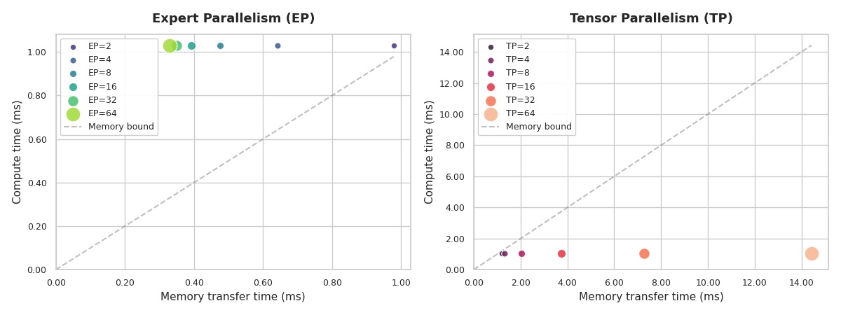
Even with TP=2 our kernel becomes extremely memory-bound! When TP increases, the time is spent on reading/writing from memory. That’s the reason why TP-only training in highly sparse MoEs is hard to spot in production training runs, and usually TP works alongside EP or PP.
So, what’s the point? How do we actually make decisions?
One natural instinct is to measure time and start optimizing the slowest kernel. But now it’s clear that raw measurements don’t tell the full story. We also need to understand the theoretical lower bound. How fast could this kernel be on the given hardware. The examples above are tools for decision-making: should we use TP or EP for this model, which kernel is damaging the end-to-end throughput the most, etc. So even when you’re sure that you can shave another 5% off a kernel in a week, don’t rush - somewhere else in the system, there might be something hiding that is running 20x slower than its theoretical optimum. Optimization time is usually the tightest constraint :)
[story continues]
tags