Why OTFS Outperforms OFDM in High-Mobility Scenarios

Table of Links

• I. Abstract and Introduction
• II. Related Work
• III. Modeling of Mobile Channels
• IV. Channel Discretization
• V. Channel Interpolation and Extrapolation
• VI. Numerical Evaluations
• VII. Conclusions, Appendix, and References

V. CHANNEL INTERPOLATION AND EXTRAPOLATION

Motivated by the fact that the channel changes much slower and thus more predictable in the D-D domain, we will in this section investigate how we can exploit the predictability for channel interpolation and extrapolation, so that the channel training overhead can be reduced.

A. Channel Interpolation with SFT

By assuming bi-orthogonality (or ignoring the ISCI, equivalently), the signal model can be simplified as

Consider a vehicular speed at 100 m/s, and the WSSUS channel model, Fig. 4 shows one realization of the wireless channel in T-F domain. In Fig. 4, the carrier frequency is

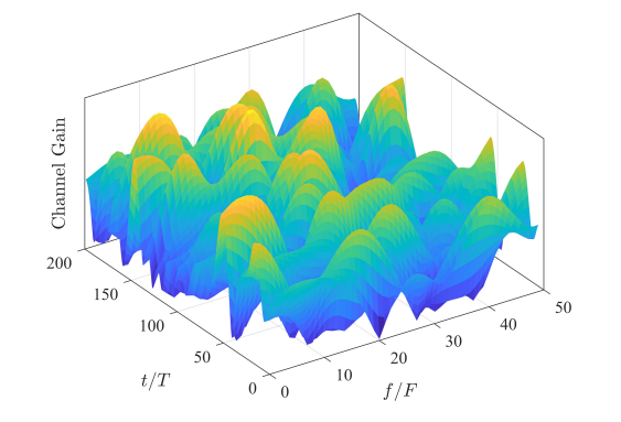
30 GHz, with a sub-carrier spacing of 200 kHz, total bandwidth of 10 MHz, and 1 ms frame length (or 200 symbols). As we can see, the channel changes very fast over both time and frequency, and the channel gains can be significantly different even between adjacent T-F slots. This example demonstrates the necessity of OTFS in highly dynamic channels.

Remarks: The above discussions hold for both discrete and continuous D-D profiles. For discrete D-D channel model, these discussions hold even when the Doppler shifts and delays of different paths are not exactly on the D-D grids in general.

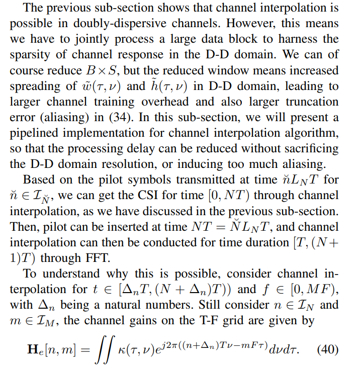
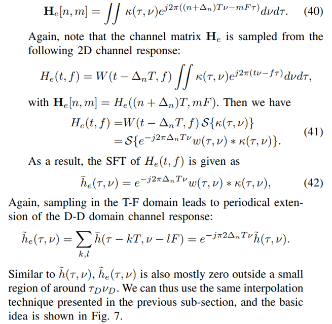
B. A Pipelined Implementation

C. Channel Extrapolation and Tracking

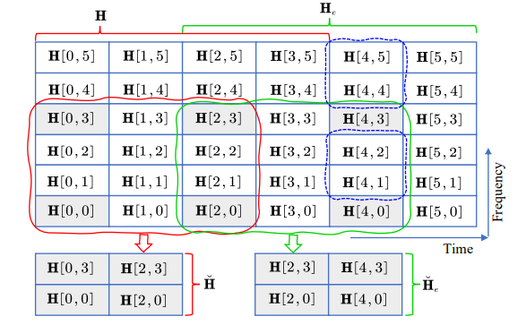
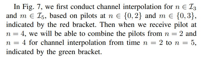
In Fig. 7, note that the data received at n = 4, i.e., encircled by the blue curves, cannot be demodulated immediately, because they have to wait for the pilot at time 4. However, based on the previous discussions, we should be able to use the previously estimated CSI for channel prediction. Specifically, we can employ the estimated CSI from time 1 and 3 for channel interpolation for time 1 to 4. From a different point of view, this is extrapolation. This also implies the possibility of channel tracking, and we further reduce the channel training overhead by inserting pilot less frequently. The idea is illustrated in Fig. 8.

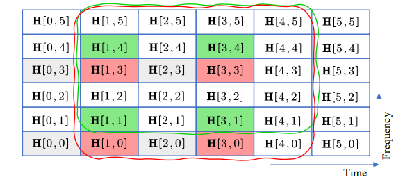
With pilot transmitted at time n = 0 and 2, frequency m = 0 and 3, channel interpolation can be conducted for time 0 ≤ n ≤ 3 and frequency 0 ≤ m ≤ 5. Then, we can use channel gains at n ∈ {1, 3}, m ∈ {0, 3}, i.e., the slots indexed by red, for channel interpolation between n = 1 and 4, encircled by red. We can thus estimate the channel gains at time 4 and 5, without waiting for the pilot. The processing delay can thus be further reduced to one symbol duration.

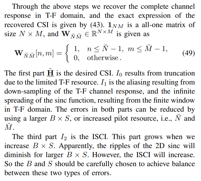
D. Error Analysis

The interpolation inevitably leads to error, because the D-D domain channel has infinitely large spread due to the finite support in T-F domain, manifested by the 2D sinc function in D-D domain. Besides, the bi-orthogonality of the signal no longer holds after going through the doubly-dispersive channel. In this sub-section, we will try to quantify the channel estimation errors resulting from aliasing and ISCI

[6] Without loss of generality, we assume that M/LM and N/LN are integers. This can be guaranteed by choosing T and F properly.